#CALC! Error In Excel – How To Fix

#CALC! error appears when an array-related calculation error is encountered in Excel. Array formulas allow you to work with several values in one formula and let you perform different calculations simultaneously.

The #CALC! error is mainly associated with dynamic arrays introduced in Excel Office 365; therefore, you will not face this error in older versions of Excel. You might also face this error whilst using the FILTER and LAMBDA functions.

To resolve this, try rewriting your formula or look at some examples below for a better understanding.

What is a #CALC! Error in Excel?

The #CALC! error mainly arises when the calculation engine of Excel faces an unexpected issue with the dynamic array formulas.

The best way to solve the #CALC! error in Excel is by going back to the basics and rewriting the formula, referring to the syntax of the functions used.

If your formula is nested, you can try utilizing the Evaluate Formula tool (from the Formulas tab > Formula Auditing group > Evaluate Formula) to find the location of the #CALC! error.

Scenarios in which #CALC! Error can Occur

Below are some scenarios of when you could face the #CALC! error along with examples and solutions.

Scenario 1: Empty Array in FILTER Function

If the formula entered returns an empty array, you would get a #CALC! error. When using the FILTER function, #CALC! error is encountered when the query results have no matching data. In such a case, since Excel can’t return an empty array so it returns a #CALC! error.

Let's try to understand this with an example.

Example 1

In this case, we are looking at the cumulative grade point average of a class of engineering students. Using the FILTER function, we will try to obtain the details of the students with a CGPA of less than 4. The formula below seems like a good place to start with:

We have mentioned the range containing the data i.e. A2:C13 in the first parameter followed by the condition C2:C13<4 that the values in column C are to be checked for values less than 4.

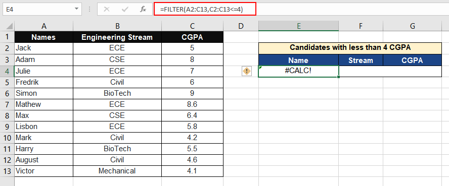
As you can see, there are no candidates with less than a 4 CGPA, and the result is empty. Therefore, Excel returns a #CALC! error. This is because we’ve missed out on the if_empty argument. This is the 3rd argument of the function. Here you need to specify what value the function should return in case it results in an empty array.

Resolution

When using the FILTER function, #CALC! error occurs when the query results in an empty array. Therefore, you must mention the if_empty condition.

To get rid of the error, we’ve taken the formula below into action:

In the given example, adding "NULL" or anything you wish to display if there is no matching result. This means that if there is no one with less than 4 CGPA, return the value NULL. Enclose the value (as we have done with NULL) in double-quotes. If you don't want any value displayed for an empty array, you can add "" which is an empty text string.

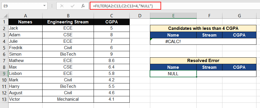
Another way to resolve the #CALC error is by adjusting the logic in the function’s first argument, so no empty value is returned.

Example 2

The data set we are using in this example contains the date and location of a list of events. For the purpose of planning, it would be helpful to know what events will take place between two dates. Now let’s see if there are any events between 1st Dec 2022 & 31 Dec 2022.

Using the FILTER function, we have come up with this formula:

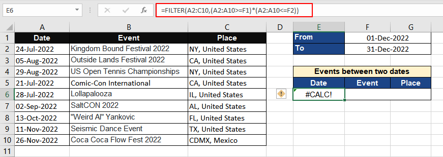
 The #CALC! error occurs as there are no events between those two dates.

Resolution

To resolve the #CALC! error, we can add a condition that if there are no events that fall in the mentioned criteria, display "No Events". This condition will be added in double-quotes as the if_empty argument. The formula is amended as follows:

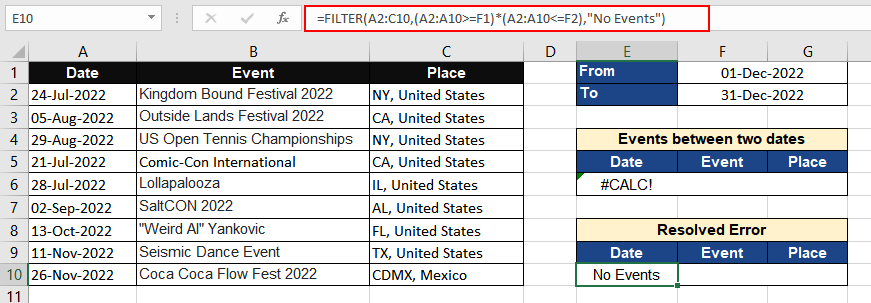
Scenario 2: Excel Web

As per the official website, when using Excel Web, you might face a #CALC! error if your calculation involves more than 10,000 cells. In Excel for the web, custom functions with references to more than 10,000 cells cannot be computed and instead result in the #CALC! error.

Scenario 3: While using LAMBDA Function

LAMBDA function allows you to create a custom Excel function. Once a LAMBDA function is created and saved, it can be inserted multiple times in a workbook.

As the LAMBDA function provides a way to create a custom function in Excel, you can develop a function for a frequently used formula and avoid copying and pasting it.

But it is important to note that it cannot be used directly without a cell reference. You will see a #CALC! error because the function needs a reference from where data can be used.

It is further explained with an example.

Example 1

You wish to convert the GBP into USD.

In general use, you would use GBP/Conversion Rate if you’re punching figures on your calculator. In Excel, if you have multiple values to convert, you would give reference to the cell containing the GBP value as done in the formula ahead:

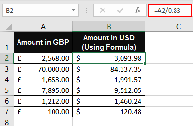
If you wish to use the LAMBDA function to carry out this conversion, you will have the advantage of being able to use the created formula throughout the workbook. To achieve that, let’s give this formula a go:

This will give you a #CALC! error as there are no references to any cells for "x". The formula has no input values to calculate with, hence it returns the #CALC! error.

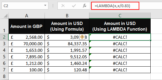
Resolution

Excel gives a #CALC! error if you assemble a LAMBDA function in a cell without giving it any references to work with. You must add parentheses with the relevant cell reference(s) to the end of your formula to call the function and provide the values to your LAMBDA function.

Let's fix the previously used formula, supplying the necessary cell reference, and see if it resolves the error for us:

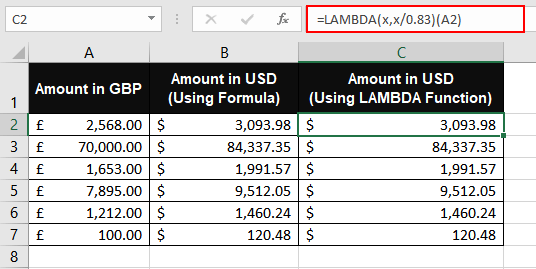
Providing the LAMBA function with A2 as the cell reference, we have successfully fixed the error! Win-win!

Example 2

Let's try using two parameters in the LAMBDA function. This is another point where the #CALC! error might occur.

Our example consists of two columns; one with the values of x, and the other with values of y. If we are to calculate the value of x²+ y², we will sum the square of x value with the square of y value. If we put this together using the LAMBDA function, we can make our own formula:

We are using the LAMBDA function to sum x raised to power 2 by y raised to power 2.

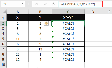
This will result in an error as you can see Excel will not understand what x and y are.

Resolution

We must give the cell reference to feed the value of x and y and resolve the error. Adding the cell references to our example formula gives us:

Adding the values from the first row in the dataset resolves the #CALC errors for us and performs the required calculation:

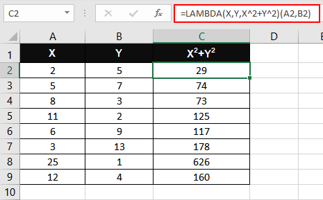
With all the above examples, hopefully, you have understood the possible scenarios where you might face the #CALC! error and how to resolve it. While you practice resolving #CALC! errors, we’ll have some more tutorials ready for you.