Excel CHOOSECOLS Function – How To Use

The CHOOSECOLS function is used to retrieve specific columns of data from an array or multiple ranges into a single new range. This function can be especially useful when working with large data sets, as it enables you to quickly and easily extract only the columns of data that you need while ignoring any unrelated data.

By using the CHOOSECOLS function, you can streamline your data analysis process and save valuable time in your work with Excel.

Syntax

The syntax of the CHOOSECOLS function is pretty straightforward and is as follows.

Arguments:

The CHOOSECOLS function accepts an array and one or more column numbers as its arguments. The details of each argument are mentioned below for better understanding.

'array' – This is a mandatory argument that accepts the original array from which we want to extract specific columns.

'col_num1' – This is also a required argument that accepts the number of the first column we want to extract from the original array.

'col_num2' – From this argument onwards, these are optional additional arguments representing the numbers of any additional columns we want to extract from the original array.

The value of the 'col_num' arguments can be a positive number or a negative number. A positive value indicates that the column should be extracted from the left side of the array, while a negative 'col_num' indicates that the column should be extracted from the right side of the array.

If we want to extract multiple columns, we can either define their numbers as separate arguments, or we can use a single argument in the form of an array constant, which lists the column numbers to be extracted.

Important Characteristics of the CHOOSECOLS Function

Some of the noteworthy features of the CHOOSECOLS function are as follows.

• The resulting array returned by the CHOOSECOLS function will have the same number of rows as the original array but only contain the selected number of columns.
• The CHOOSECOLS function spills its results into the required rows and specified columns.
• The column numbers in the col_num argument must be integers, and they should correspond to valid column positions in the original array.
• If any of the values of the col_num arguments in the CHOOSECOLS function have an absolute value of zero or exceed the number of columns in the array, Excel will return a #VALUE error.

Examples of CHOOSECOLS Function

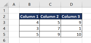
Let's begin by understanding the basic functionality of the CHOOSECOLS function. Here we have a simple dataset of random numbers in three columns. We are trying to extract columns 1 and 3 from the larger array.

The formula used will be as follows.

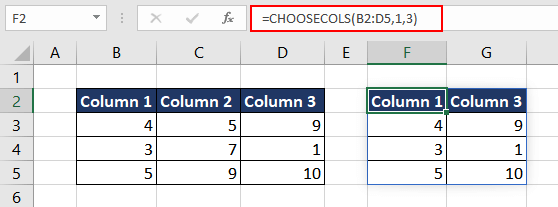
The formula takes the range B2:D5 as its first argument, which represents the entire dataset. The second argument, "1" refers to the first column of the dataset (i.e. column B) while the third argument, "3", refers to the third column of the dataset (i.e. column D). Therefore, the output of this formula is a new range or array that includes only the data from columns B and D of the original dataset, with all other columns omitted.

Now that the basic functionality of the CHOOSECOLS function is clear, let's move on to some applications and examples of the function.

Example 1 – Extracting Two Columns Using CHOOSECOLS Function

In this example, we have a dataset that contains information about a company's sales over the past year. The dataset includes columns for the salesperson's name, the date of the sale, the product sold, the quantity sold, and the total sales amount. Now, for a quick analysis, we wish to create a summary report that shows the total sales for each salesperson.

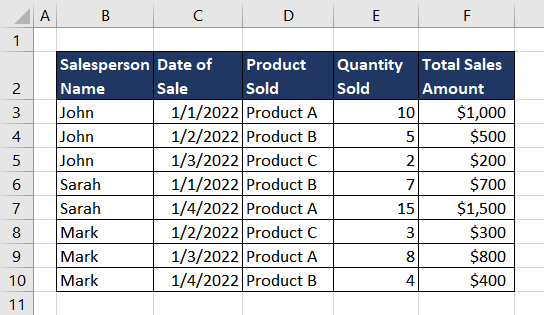
In order to create the intended summary report, we only require columns B and F. The formula used will be as follows.

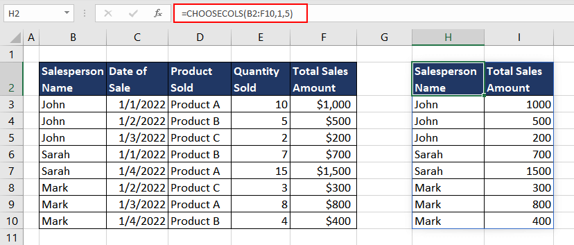
A simple application of the CHOOSECOLS function allows us to limit the data as per our requirements.

Example 2 – Extracting Last Column Using CHOOSECOLS Function

In this example, we have downloaded daily share prices for a company we want to invest in from the internet. For analysis, we wish to extract data from the last month to calculate the average stock price of the latest month.

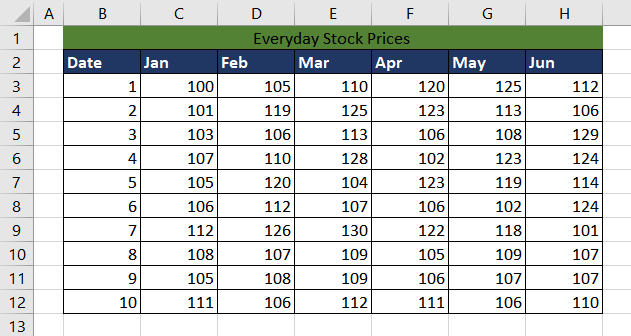
We can use the CHOOSECOLS function to extract columns B and H which contain the data for the last month along with the date. One way to do so is to count the total columns manually and then use the first and last column number as the input value for the col_num argument. The formula used will be as follows.

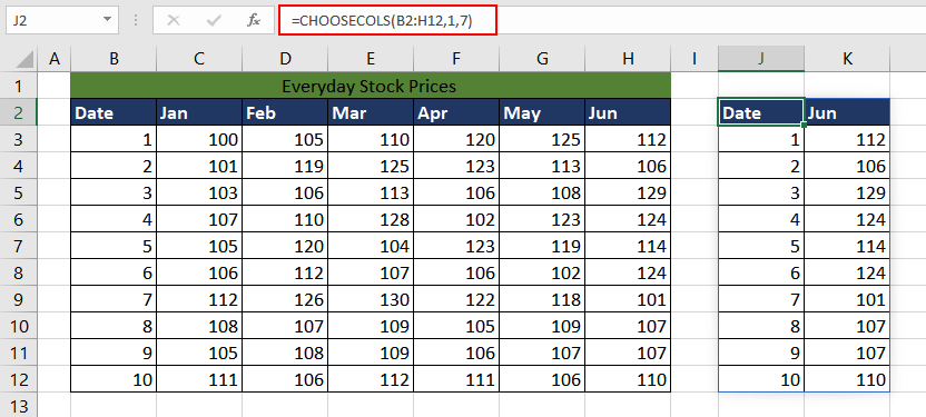
But if we are dealing with a large dataset, counting the number of columns is inefficient. Instead, we can use a negative input value for col_num to ensure that the CHOOSECOLS function counts from right to left. The updated formula will be as follows.

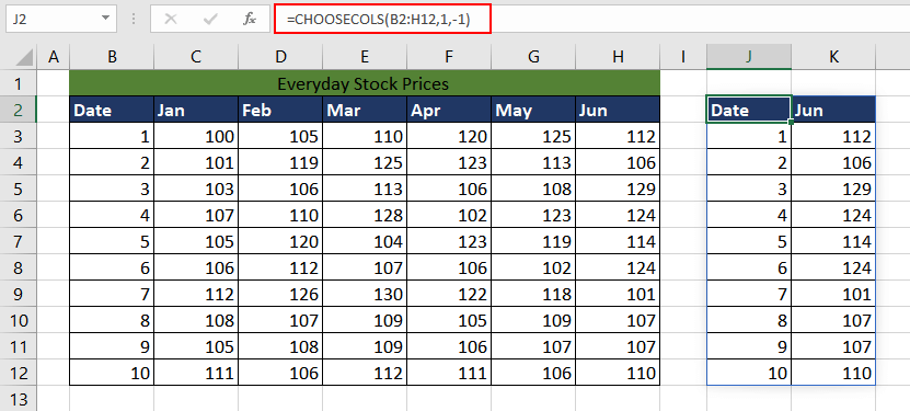
Now you can simply calculate the average price as intended.

Example 3 – Reversing Order of Columns Using CHOOSECOLS Function

In this example, we have a dataset that contains the monthly revenue figures for a company for the last 5 years, and we want to analyze the trend in revenue over time. The dataset shows the monthly

revenue figures for a company from 2018 to 2022, and the data is arranged in columns, with each column representing a different year and each row representing a different month.

For better analysis, we wish to see the most recent data first and reverse the order of columns.

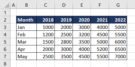
Using the CHOOSECOLS function along with other Excel functions, we can flip the array of monthly revenue figures horizontally so that the columns are in reverse order, i.e., from the most recent year to the oldest year. This will allow us to analyze the revenue trend over time more efficiently.

The approach we will use to flip the array will be to use the SEQUENCE function to determine the order of columns for the second argument of the CHOOSECOLS function. To reverse it, we will multiply each number of the sequence by -1. Let's understand it step by step.

We will first use the COLUMNS function to count the total number of columns in the range. The formula used will be as follows.

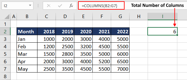
Now we will use the SEQUENCE function to generate a sequence of numbers from 1 to the number of columns in the range B2:G7, which is already calculated by the COLUMNS function. The formula used will be as follows.

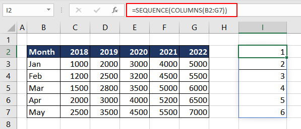
This sequence will be used as the second argument of the CHOOSECOLS function, indicating the order of the columns in the output. But as we wish to reverse the order, we will multiply the sequence with -1, effectively reversing the order of the columns. The formula used will be as follows.

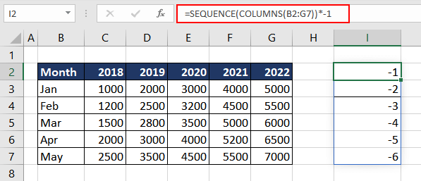
The resulting sequence will enable the CHOOSECOLS function to return the columns from right to left, therefore flipping the array. The final formula to be used is as follows.

The reversed orientation of the input data will now make it easier for trend analysis.

Now, what if the columns to be retrieved from a dataset are entered by the user and are in text format? Let's explore this scenario in the next example.

Example 4 – Extract Columns based on String with Numbers

Let's say we have a database of customer orders with several columns of data, including the customer name, order number, order date, order total, and order quantity. Depending on the intent, the user can extract any combination of columns for their analysis.

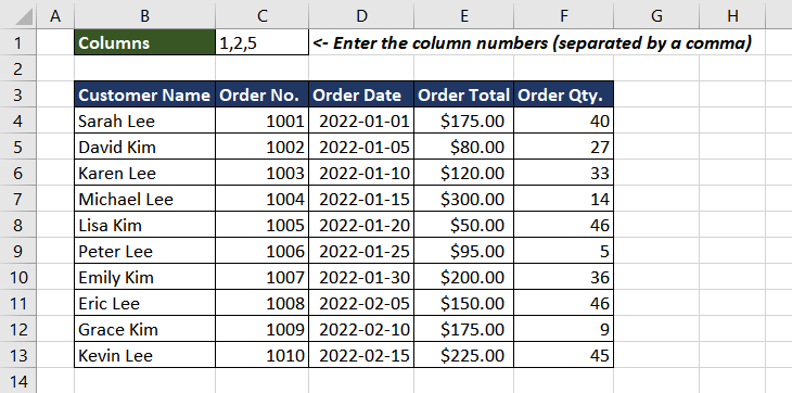
Suppose the team who delivers the orders wants the customer's name, order number, and order quantity. They can enter the column numbers in cell C1 and using the CHOOSECOLS function, we can extract the required columns.

As the user input data is in text format and is a string, first we need to split the text string in cell C1 containing the column indexes of the desired data into an array of numbers, and then pass that array to the CHOOSECOLS function to select the appropriate columns.

To split the text string "1,2,5" into an array of three numbers (1, 2, and 5) using the TEXTSPLIT function, the formula used will be as follows.

We are also multiplying the return value by 1 to convert the text format to numerical format.

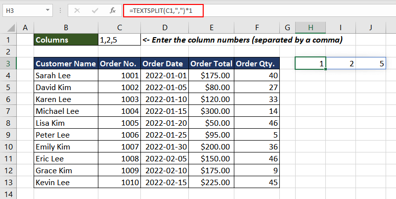
Now that we have the column numbers, we will use these values as the input data for the col_num argument. The formula will be as follows.

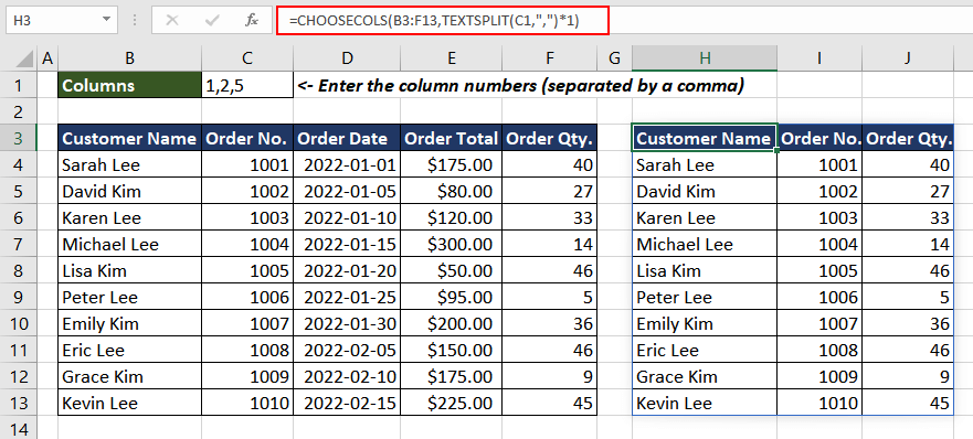
Now any user can extract the desired columns from the dataset.

Example 5 – Extracting Columns from Multiple Ranges using CHOOSECOLS Function

Assume that you work for a sales company, and you have sales data for each of your salespeople in three different regions: North, South, and West. The data for each region is stored in separate ranges as shown below.

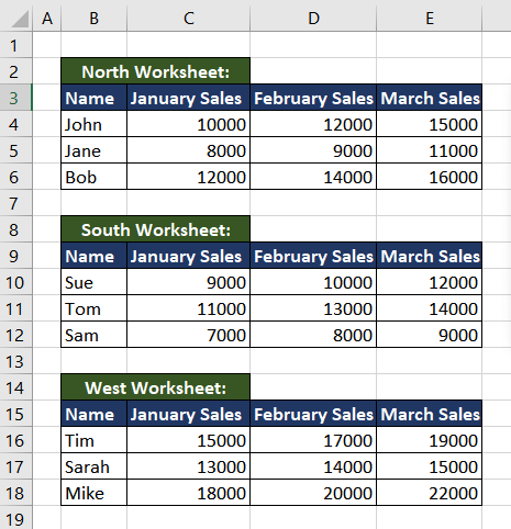
Now we wish to create a summary report that shows the total sales for each salesperson across all three regions for January. To do this, we need to extract the January sales data for each salesperson from each of the three cell ranges and combine them into a single table.

To combine the cell ranges, we will first use the VSTACK function and then extract columns 1 and 2 from the entire range. The VSTACK function in Excel is used to vertically stack the values or ranges of data from multiple columns or ranges into a single column or range. The formula used to combine the ranges is as follows.

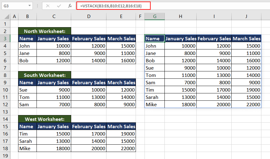
Now that we have the cell ranges combined, using the CHOOSECOLS function, we will extract the intended data. The formula used will be as follows.

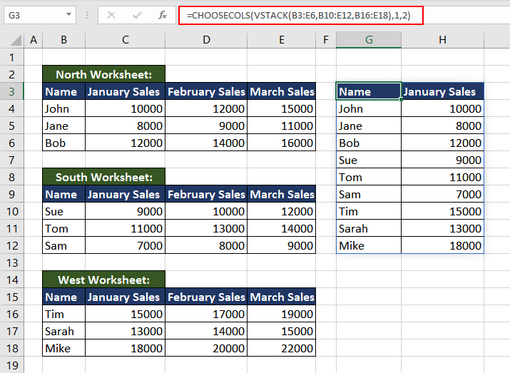
CHOOSECOLS VS CHOOSEROWS Function

The CHOOSECOLS function returns a new array containing only the selected columns, while the CHOOSEROWS function returns a new range of cells containing only the selected rows.

The key difference between the two functions is in how they interpret their arguments. CHOOSECOLS accepts the column numbers to be extracted while the CHOOSEROWS function accepts row numbers to be extracted as an argument. Let's better understand it using an example.

Here we have an array of random numbers containing 5 rows and columns.

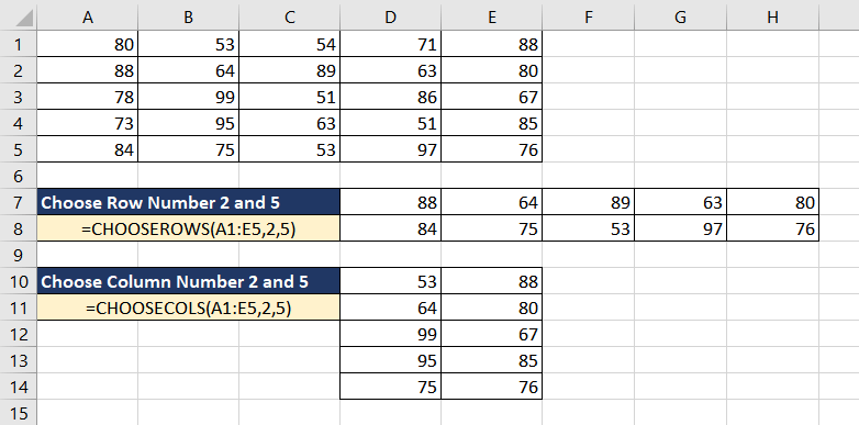
In the first case, we are trying to extract row number 2 and 5 from the array. The formula used will be as follows.

It simply returns data from rows 2 and 5, resulting in a new array.

In the next case, we are using the CHOOSECOLS function to extract column number 2 and 5. The formula used will be as follows.

So, depending on whether you want to select specific columns or rows of data, you would use either the CHOOSECOLS or CHOOSEROWS function to accomplish your goal.

Practice and explore new ways to use the CHOOSECOLS function while we bring to you another useful Excel function to cut into.