Excel CHOOSEROWS Function – How To Use

The CHOOSEROWS function in Excel extracts the specified rows from a given range of cells or arrays. The function is especially useful when we need a smaller dataset from large data based on row numbers.

The CHOOSEROWS function returns a new single array that contains the rows we want. It makes data analysis and extraction faster as it helps pull out the data we need, without having to manually search through the entire data set.

Syntax

The syntax of the CHOOSEROWS function is as follows.

Arguments:

The CHOOSEROWS function accepts the following arguments:

'array' – This is a mandatory argument that contains the input array from which we want to select the rows. It can be a range of cells, an array constant, or an array formula.

'row_num1' – This argument is also mandatory and specifies the first-row number to be selected from the array.

'row_num2' – From this argument onwards, all are optional arguments that include the additional row numbers to be selected from the array. We can include as many row numbers as we need, separated by commas.

The row_num argument in the CHOOSEROWS function can either be a positive or negative value, where a positive value indicates that the row should be extracted from the top of the array, while a negative value indicates that the row should be extracted from the bottom of the array. To extract multiple rows, we can either define their row numbers as separate arguments, or we can use a single argument in the form of an array constant that lists the row numbers to be extracted.

Important Characteristics of the CHOOSEROWS Function

Some of the noteworthy features of the CHOOSEROWS function are as follows.

• The CHOOSEROWS function returns a new array or range of rows based on the row numbers provided as arguments. The returned array will have the same number of columns as the original array.
• The CHOOSEROWS function returns a #SPILL! error if the resulting array spills in the range that already contains data.
• If the mandatory arguments are left empty, the CHOOSEROWS function throws a #VALUE! error.
• If the value of the row_num is greater than the number of rows in the array or is set to 0, the CHOOSEROWS function returns a #VALUE! error.

Examples of CHOOSEROWS Function

To understand the basic functionality of the CHOOSEROWS function, we will begin with a simple example and then move on to different applications of using the said function.

Example 1 – Simple Use of CHOOSEROWS Function

Here we have a simple dataset containing day-wise sales from our new online business. We wish to create a summary report containing daily sales data for the first 3 days.

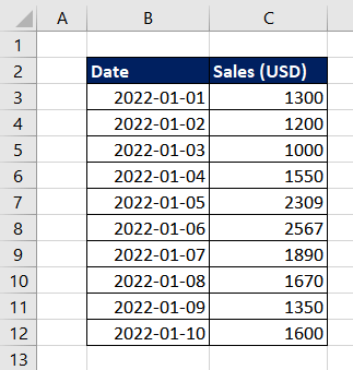
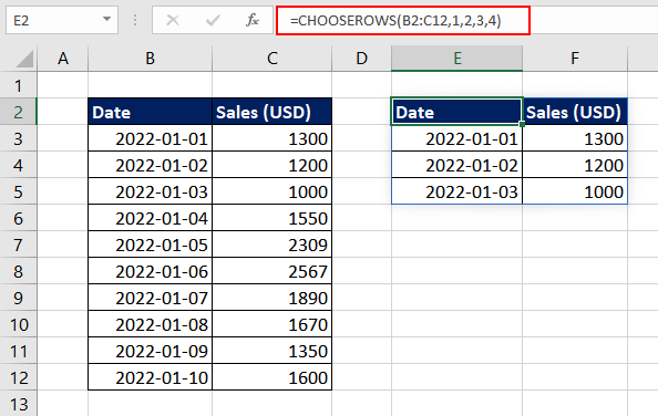
Now, to extract the sales data for the first 3 days, we will use the corresponding row numbers in the CHOOSEROWS function and the range B2:C12 as the first argument, representing the entire dataset. As the first row contains the headers, we will include that too. The formula used will be as follows.

The formula has returned rows 1 to 4 from the dataset:

Another way of specifying the rows to return is to use the row numbers as an array constant. The formula will look like this.

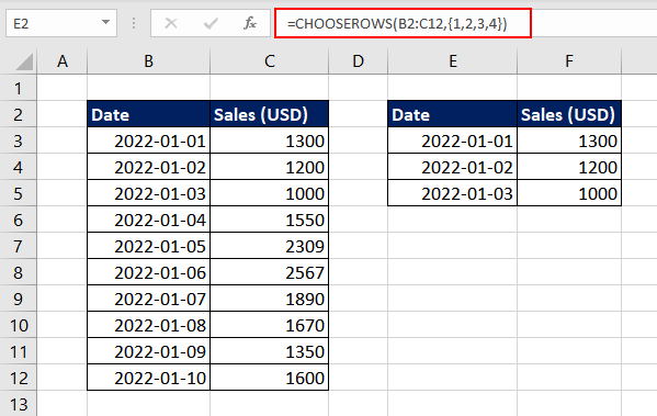
Example 2 – Extracting Last Few Rows Using CHOOSEROWS Function

Here in this example, we have a dataset that contains stock price data for the past few days, and we want to extract the last 3 trading days to analyze the stock's performance.

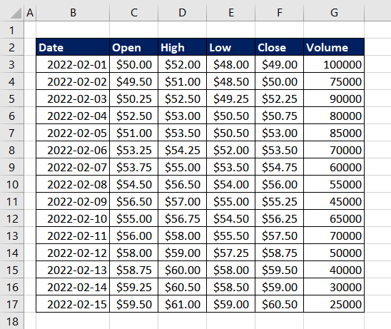
As the data is sorted in chronological order, with the most recent prices at the bottom of the dataset, there are two ways to extract the last 3 rows. One way is to count the total number of rows and then manually enter the row number. The formula used will be as follows.

We are trying to extract the first row which contains headers for each column in the dataset. Then, as intended we manually entered the last three row numbers.

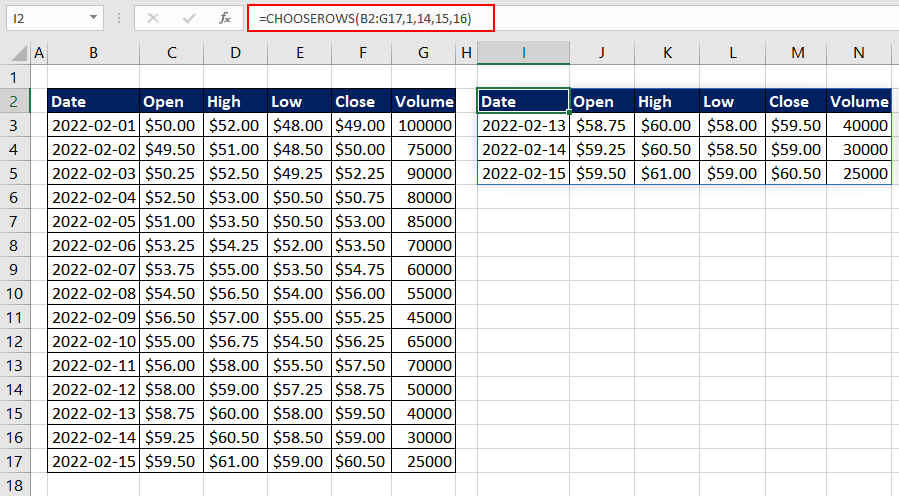
This is not an efficient way if the dataset is large. Instead, we can make use of one of the characteristics of the CHOOSEROWS function. We can use negative values for the row_num argument so that the function counts from bottom to up. The formula will be as follows.

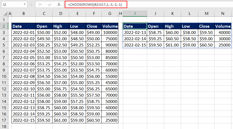
Now, no matter how large the dataset is, you can easily extract the last few rows using the negative values for the row_num argument. If we wish to reverse the order of the rows, the formula used will be as follows.

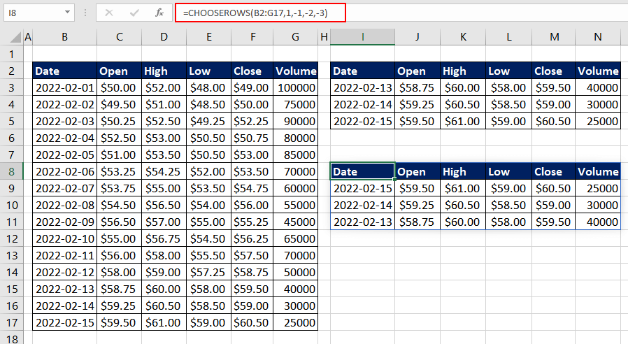
Example 3 – Reversing Row Order Using CHOOSEROWS Function

Suppose we have a list of sales data where each row represents a sale and the columns contain details about the sale, such as the date of the sale, the customer name, the product or service sold, the sale price, and the quantity sold.

If we want to analyze the sales data and present it in a report or chart, it would be best to reverse the order of the rows to show the most recent sales first. That would allow us to focus on the most recent sales and identify any trends or patterns over time.

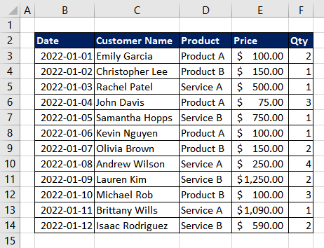
Using the CHOOSEROWS function in combination with SEQUENCE and ROW functions, we can easily reverse the order of rows as required. The ROWS function counts the total number of rows in the given array. The formula used will be as follows.

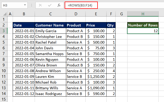
Now that we have the number of rows, we can use the SEQUENCE function to generate an array of sequential numbers, with the number of rows in the range B3:F14. The formula used will be as follows.

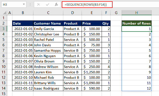
The next step is to multiply each number in the array by -1, effectively reversing the order of the numbers. The updated formula will be as follows.

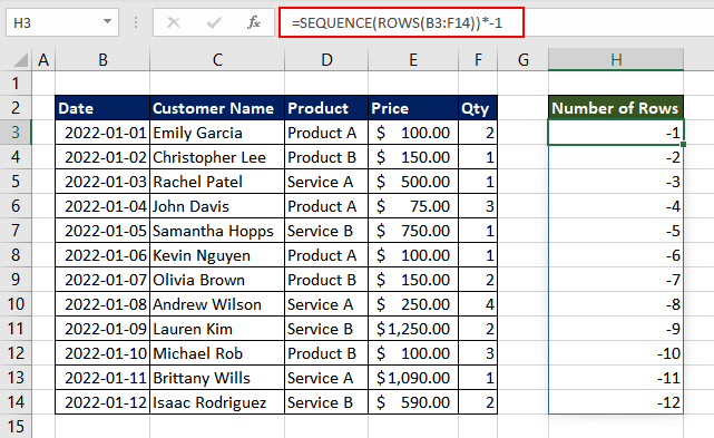
Finally, we can use the CHOOSEROWS function to select the rows from the range B3:F14 in the order specified by the array generated by the above-mentioned SEQUENCE function. As the values from the SEQUENCE function are all negative, the CHOOSEROWS function starts selecting rows in reverse order, which will flip the array vertically. The formula used will be as follows.

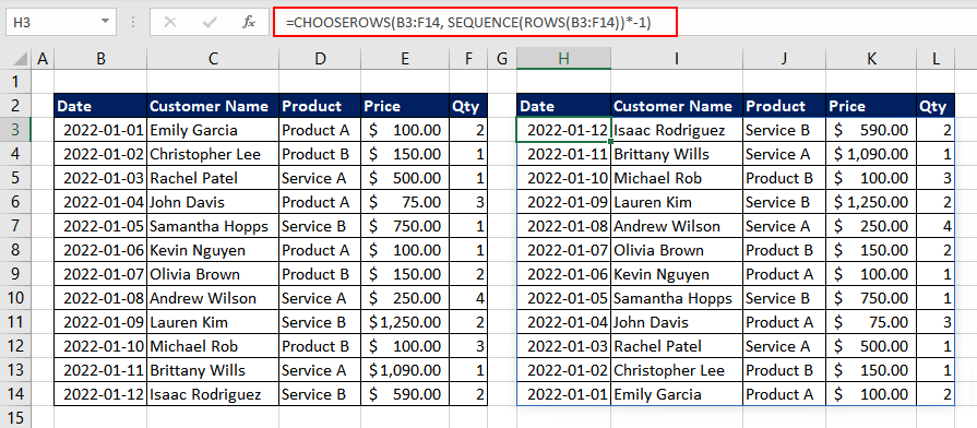
The final result is a range that is identical to the original range B3:F14, but with the order of rows reversed as required.

Example 4 – Randomly Choosing Row from Multiple Arrays Using CHOOSEROWS Function

Here in this example, we have a dataset that contains employee data who joined in four quarters of the year. Each quarter has a separate table with columns for employee name, department, salary, start date, and office location. We wish to randomly select one employee to attend an upcoming conference.

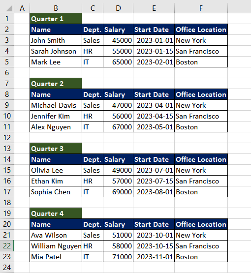
To obtain particular rows from multiple non-consecutive ranges, we can merge all the tables using the VSTACK function and subsequently input the merged range into the CHOOSEROWS function to retrieve the chosen rows. The formula used will be as follows.

The VSTACK function takes the given cell ranges and stacks them vertically into a single, longer range.

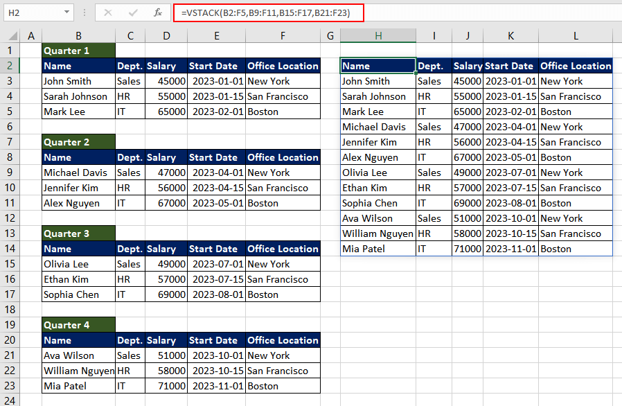
Now that we have a combined range, this will act as an input value for the first argument of the CHOOSEROWS function which is an array. For the second argument, as we wish to randomly choose one row, we will use the RANDBETWEEN function to generate a random row number between row number 2 and the total number of rows.

We can calculate the total number of rows in the resulting array by using the ROWS function and passing the output of the VSTACK function as its input. The final formula to generate a random row number will be as follows.

Now, combining both to get our final CHOOSEROWS function, which will be as follows.

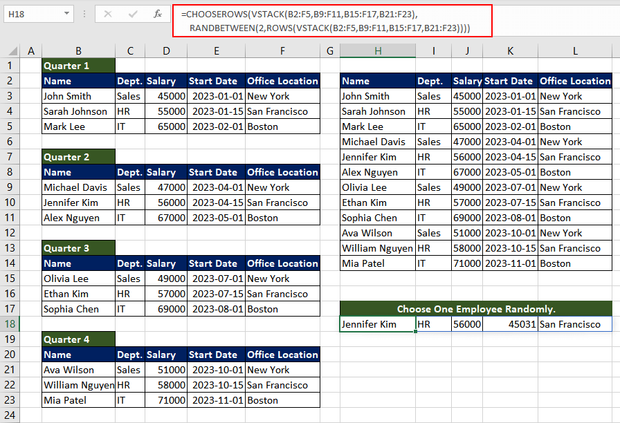
Don't be intimidated by the length of the formula, it's actually quite simple if you understand it correctly. Try it on your own and discover a new application.

In the above example, we randomly choose a row. However, if the user provides row numbers in text format to be extracted, the process may differ. Let's understand it using an example.

Example 5 – Extracting Rows Based on String Containing Row Number

In this example, we are planning a holiday. Just to check the weather for the upcoming days, we downloaded the data for 16 days. The dataset contains the date, and day of the week along with the type of weather and temperature. Now, we can simply extract data for a few days and plan our vacation.

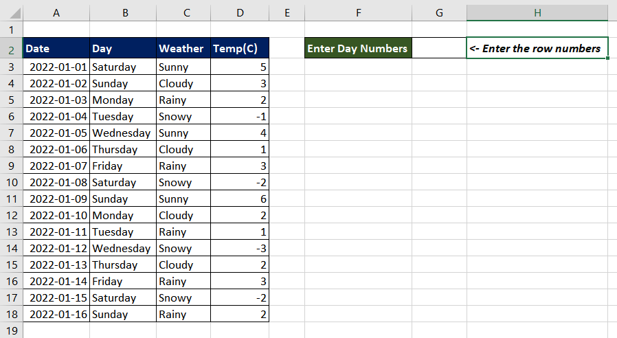
We can enter the day numbers in cell G2 and create a smaller dataset using the CHOOSEROWS function. As the data entered will be in text format, we first need to convert the text string which contains the row numbers of the desired data, into an array of numbers. We can then use that array as an argument to the CHOOSEROWS function to extract the corresponding rows from the dataset. In this case, we wish to extract the weather data for the next two weekends which is day 1,2,8,9.

To split the input comma-separated list, the we will make use of the TEXTSPLIT function as follows.

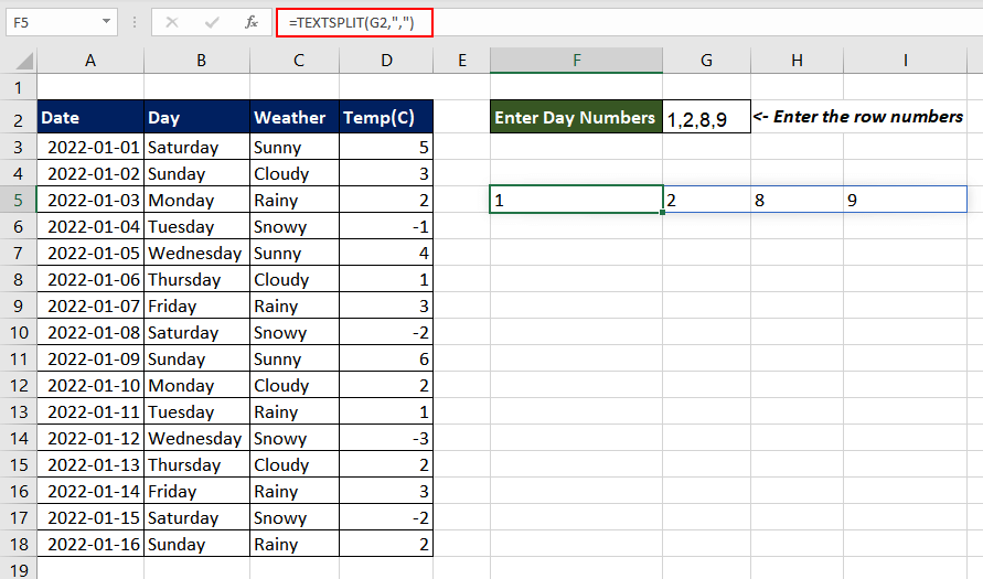
As the resulting data is in text format indicated by the left alignment in the cell, we will simply multiply it by 1, which will give us the same data in numeric format. The updated formula will be as follows.

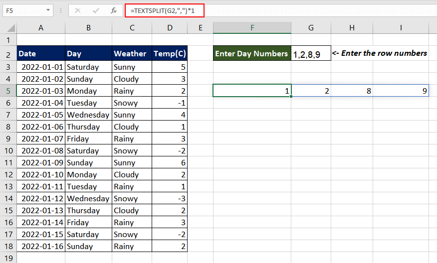
Now that we have a numeric array to select rows, we will use the CHOOSEROWS function to select the rows from the range A3:D18. The formula used will be as follows.

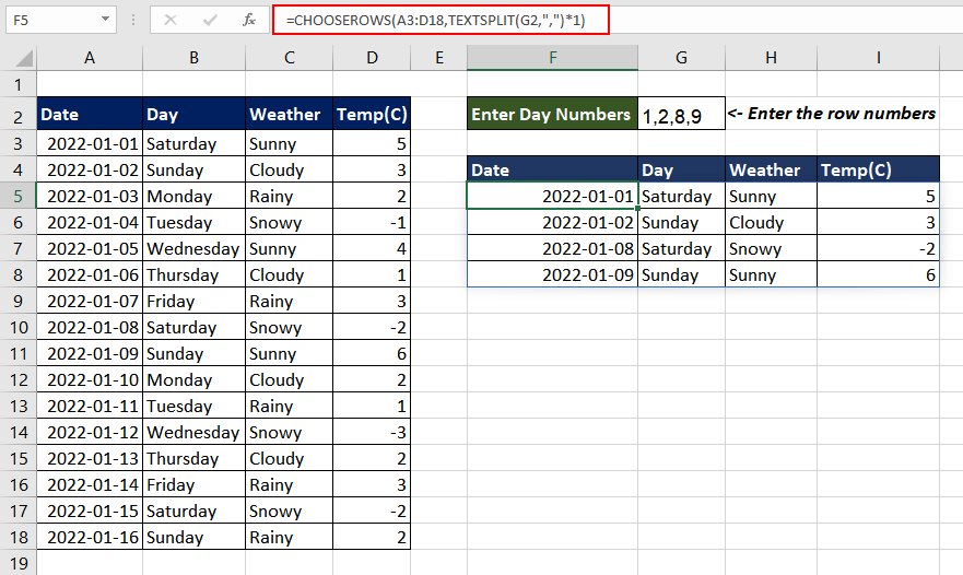
Now that we have the required data, we can plan which weekend is more appropriate for a vacation.

CHOOSEROWS VS CHOOSECOLS Function

The CHOOSEROWS function returns a new array containing the specified rows, while the CHOOSECOLS function returns a new cell range with selected columns.

Let's understand it better with an example.

Here we have a dataset (B2:E5) that consists of a table with four columns and three rows. We will now try to extract row and column numbers 1 and 3. The formula used will be as follows.

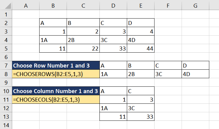
The CHOOSEROWS formula extracts the specified rows from the given data range, B2:E5, and returns a new range containing rows 1 and 3 of the original data range. The CHOOSECOLS formula, on the other hand, extracts the specified columns from a given data range and returns a new range containing columns 1 and 3.

Both CHOOSEROWS and CHOOSECOLS functions allow us to extract specific rows or columns from a cell range or array, based on an index number or array of index numbers.

Practice the function and discover new ways to make full use of it, while we haul another interesting Excel function to improve your data analysis and productivity.