The CODE function is an Excel text/string function that returns the numeric code associated with the given character.
The returned numeric code corresponds to the character set used by your computer (Windows OS uses the ANSI character set, whereas Mac OS uses the Macintosh character set).
When more than one character or a string is passed to the function, the CODE function will return the numeric value of the first character.

Syntax
Following is the syntax of the CODE function:
=CODE(text)Arguments:
'text' – The text against which the numeric code will be returned. This argument is mandatory, and it accepts a character, string, or any function that returns a text value.
Important Characteristics of the CODE function
- Although it is a text function and the input argument must be a text value, the return value is numeric.
- If the text argument is left blank, the CODE function will return a #VALUE error.
- Other than numbers, all characters or text strings must be entered enclosed in double-quotes in the text argument or the function will return a #NAME? error.
- The return value of the CODE function might vary with the operating system. Windows OS uses the ANSI character set while MAC/Apple OS works on the Macintosh character set.
- The CODE function returns the ANSI code for a character and will return values from 1 to 255 (the first 32 characters being unprintable control codes).
Examples of CODE Function
Let's see the straightforward use of the CODE function first.
In this example, Column B lists various inputs like alphabets (both lowercase & uppercase), numbers, strings, and special characters. In column C, we are passing these inputs to the CODE function using the formula:
=CODE(B3)As we can see, the result in column C is the ANSI code corresponding to the input. For instance: the ANSI code for A is 65, and hence the CODE function returns 65 in the first instance. Likewise, the formula returns the ANSI code for all the other input values listed below.
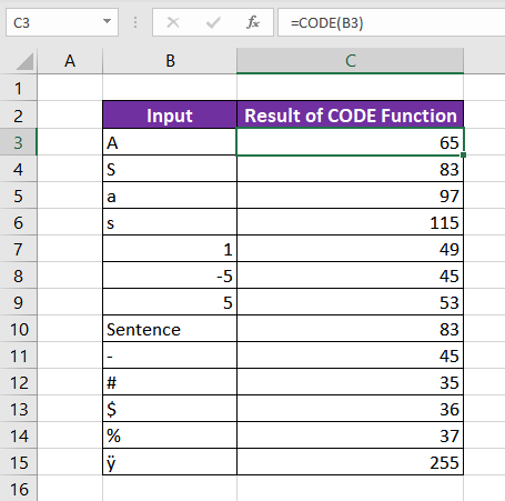
If you observe carefully, you will note that the results for cells B8 and B9 differ. This implies that the CODE function returns different results for 5 and -5. This difference can be explained by the fact that the CODE function returns the numeric value corresponding to the first character only.
The same is true in cell B10, where the value returned corresponds to the first character 'S'.
Now that the basic usage of the CODE function is clear, let's combine it with different Excel functions in the examples below.
Example 1- Remove Unwanted Characters from Beginning of Text
In this example, a friend sent you a list of books to read for the summer. Upon downloading, there
were unwanted characters in the data, which made it difficult to read. It would be a troublesome task to remove the characters manually, so instead, use the CODE function to your advantage.
The downloaded data in column B (name of the books) looks like this.
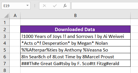 As we can see, the unnecessary character is at the beginning of each book name and is repeated multiple times in a cell. Using the SUBSTITUTE function, we can easily replace the character with an empty string. The formula used will be as follows
=SUBSTITUTE(B3,"!","")We can also use the CHAR function instead of the character. CHAR function accepts the ANSI code of a character and returns the subsequent character. In this case, the formula used will be as follows. Note that =CHAR(33) returns "!".
=SUBSTITUTE(B3,CHAR(33),"")But the problem is that the character is different in each book name. So, the above formula will not work for all books. Let's figure out another way that can be used for all the books irrespective of the unwanted character.
As the unwanted character is the first character in each book name, let's put that to good use. Using the LEFT function, we can extract the character repeating itself. So, the formula goes as follows
=LEFT(B3)The LEFT function returns the first character when the second optional argument is left blank. Now, that we have the character to be removed. Using the CODE function, we will determine its ANSI value, which in turn will be used in the CHAR function. The formula goes as follows
=SUBSTITUTE(B3,CHAR(CODE(LEFT(B3))),"")Here, we are utilizing CODE and CHAR functions to provide a code dynamically, using the first character in the cell, rather than directly providing character 33 to SUBSTITUTE.
Example 2 – Removing Currency Sign to Calculate the Sum
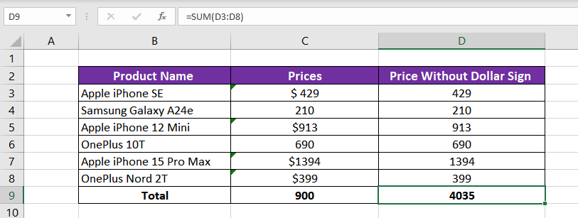
Suppose we ordered a few mobile phones and received the price list. We now wish to add the prices of all the mobile phones, but few prices are mentioned with the dollar sign ($).
When we tried adding all, Excel did not include the ones with the dollar sign as they are in text format – shown in cell C9.
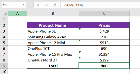
To resolve this, we must remove the dollar sign from the prices in column C and then convert it into a numeric value. So, the logic we will use to get the desired data is as follows.
If the first character of the cell value is "$", then substitute the dollar sign with an empty string and convert the value in the cell to numeric format using the VALUE function. If not, then let the cell content remain the same.
Let's break down the logic in Excel formulas. To extract the first character from the cell, we will use the LEFT function as follows.
=LEFT(C3)Now, we will compare the extracted character with the ANSI code of the dollar sign which is 36. The CODE function combined with the LEFT function will be written as:
=CODE(LEFT(C3))=36If there is a dollar sign present, it must be removed or replaced with an empty string and then the entire value of the cell (the price of the mobile phone) must be converted to numeric format. This can be done with the following formula:
=VALUE(SUBSTITUTE(C3,LEFT(C3),""))Using the SUBSTITUTE function in C3 to replace the first character with an empty string (""). Then, wrapping the entire result in the VALUE function. Finally, using the IF function to combine everything, the final function looks like this.
=IF(CODE(LEFT(C3))=36,VALUE(SUBSTITUTE(C3,LEFT(C3),"")),C3)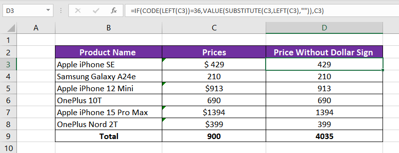
You can now calculate the sum of mobile phone prices (shown in cell D9) as there is no dollar sign, and all the values are in numeric format.
Example 3 – Add Question Marks Where Missing
In the following example, we will again use the CODE function to make our job easier and faster. We have a set of most asked interview questions in this data set in column B, but few of them do not end with a question mark (?). Not very presentable, right?
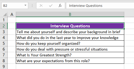
To ensure that all the interview questions end with a question mark, we will use the CODE function combined with other Excel functions such as IF, RIGHT & CONCAT. The logic we will use to get the desired result is to check if the input string contains a question mark at the end. If yes, we will just use the existing string; if not, we will add a question mark at the end.
Let's compile it in Excel format using functions.
To check the last character of the string, use the RIGHT function, which extracts the given number of characters from right to left. If the second optional argument is left blank, by default, it extracts the last character. So, the function goes as follows:
=RIGHT(B3)Combining it with the CODE function, we will compare if the last character is a question mark. The ANSI value of '?' is 63. So, the formula used will be:
=CODE(RIGHT(B3))=63As we can observe, there are several questions where the result is FALSE (no question mark present). We will use the IF & CONCAT function to fix this.
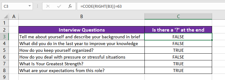
CONCAT function is used to join texts. So, in cases where the result is FALSE (indicating the absence of a question mark), the approach will be to join the input text with a question mark at the end. The formula will be as follows.
=CONCAT(B3,"?")Combining all the above formulas to get our final version
=IF(CODE(RIGHT(B3))=63,B3,CONCAT(B3,"?"))
Now, it looks presentable and gives a good impression. The next example is our favourite, so make sure that you are on the Excel workbook to try it.
Example 4 – How to Autofill A to Z in Excel
We all know the easiest trick in Excel is to autofill numbers in a column. If we wish to add 1-40, we can simply write 1 in the first cell and 2 in the next one to suggest a pattern, and then, after selecting the two, drag & fill the cell till 40. Pretty neat, right?
But, how to autofill alphabets in Excel? Use the CODE and CHAR functions to impress your co-workers. The logic used is similar to what we use in auto-filling numbers which is adding 1 to the previous one. Just that in this case, we will use the CODE function to convert the preceding letter to the ANSI code, add 1 to it, and convert it into the corresponding character.
The ANSI code of 'A' is 65, for 'B' it is 66, and so on till 'Z', which corresponds to 90. So, start with inserting 'A' in the first cell B3 and apply the CODE function to it.

Adding 1 to the code value of A, the function will progress to
=CODE(B3)+1Now, getting to our desired result, that is the next alphabet 'B', we will use the CHAR function, which is our final step.
=CHAR(CODE(B3)+1)The CHAR function will take the code from the CODE function (65+1 = 66) and return the character against that code, "B" in this case.

Drag the fill handle till you get your last alphabet, 'Z'.
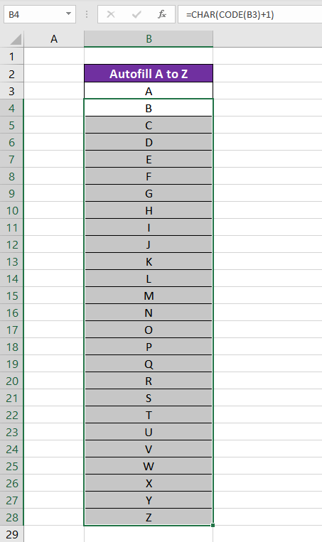
You can repeat the same logic for lowercase alphabets. Type 'a' in the first cell and repeat the formula.
CODE vs CHAR Function
The reverse of the CODE function is the CHAR function. CODE function returns the numeric value of the character, whereas the CHAR function returns the character associated with the given number.
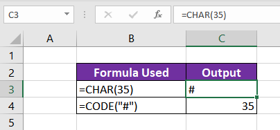
As shown in the example above, CHAR(35) returns the character '#', and CODE("#") gives 35.
That brings our CODE function saga to an end. Try out each of these examples on your own, and once you feel confident using these formulas, come back to us and we'll make sure we have the next function ready for you to learn. Until then – stay curious!


