Excel DROP Function – How To Use

The DROP function removes the specified number of rows or columns from the start or end of the array. The function is highly useful for removing headers, outliers, or any unnecessary data.

The DROP function accepts the number of rows or columns to exclude and returns a new array or dataset. Understand the function and make full use of it while data cleaning or filtering.

Syntax

The syntax of the DROP function includes three arguments and is as follows.

Arguments:

The DROP function accepts one required and two optional arguments. The details of each are mentioned below.

'array ' – This is a mandatory argument that includes the cell range or array from which the row(s) or column(s) are to be removed.

'rows' – It is the number of rows that are to be removed or dropped from the input array. It is an optional argument; if left empty, the default value is set to 0. A positive value of the rows argument indicates that the row(s) will be removed from the top of the array, while a negative value suggests that the row(s) will be removed from the bottom of the array.

'columns' – It is also an optional argument and specifies the number of columns to be removed. If left empty, the default value is set to 0. If the value of the columns argument is positive, the column(s) will be removed from the beginning of the array. On the other hand, if a negative value is provided, the column(s) will be removed from the end of the array.

Important Characteristics of the DROP Function

One of the basic characteristics of the DROP function is that it results in a new array that spills into the worksheet. Some of the other noteworthy features of the DROP function are as follows.

• If the array argument is left empty, the DROP function throws a #VALUE! error.
• When the input array is empty, the resulting array includes 0 values depending on the rows and columns.
• If the number of rows to be removed is more than the rows in the input array, the DROP function returns a #CALC! error. The same error is reported if the total number of columns to be removed is more than the columns in the given array.

Examples of DROP Function

Let's begin by populating different values for all three arguments of the DROP function to gain a better understanding of its fundamental nature. Here, we have taken a sample array (B1:D2) that contains two rows and three columns.

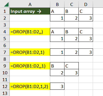
In the first instance, we are checking the default nature of the DROP function, which is when both optional arguments are left empty. As the value of both the rows and columns argument are 0, the function does not remove anything and returns the original array.

The second example showcases the instance when there is an input value for the rows argument, but the columns argument is left empty. The DROP function, in this case, removes one row from the beginning and does not drop any columns. The resulting array contains the remaining row.

In the third case, the DROP function excluded the first column from the left and did not remove any rows, as the argument is left empty.

The last case is a classic example where we are trying to drop 1 row and 2 columns from the input array. As they are both positive values, the function counts the rows and columns from the beginning and removes them.

Now that the basic functionality of the function is clear – let's move on to some practical examples.

Example 1 – Simple Use of DROP Function

Suppose we have an employee satisfaction survey dataset that includes responses from employees on two questions. The dataset includes information such as employee ID and the time stamp. Ideally, such data must not contain information leading back to the employees. To resolve that, we want to remove a few rows and columns to use the data for further analysis.

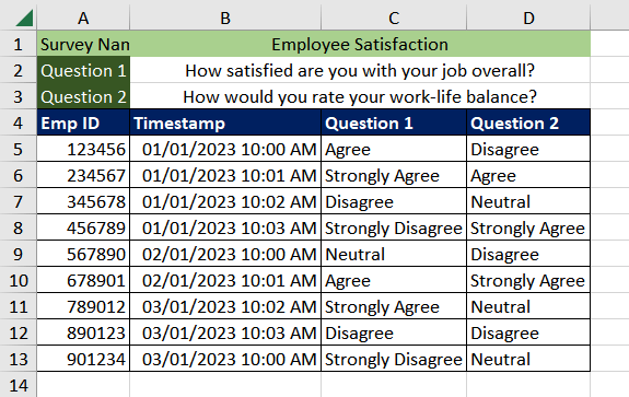
As we can see, the first three rows contain details about the survey title and the questions asked, while the first two columns include employee ID and the time stamp.

One option is to manually delete the selected rows and columns, which is highly inefficient. Instead, we can use the DROP function to exclude the first 3 rows and first 2 columns from the dataset A1:D13. The formula used will be as follows.

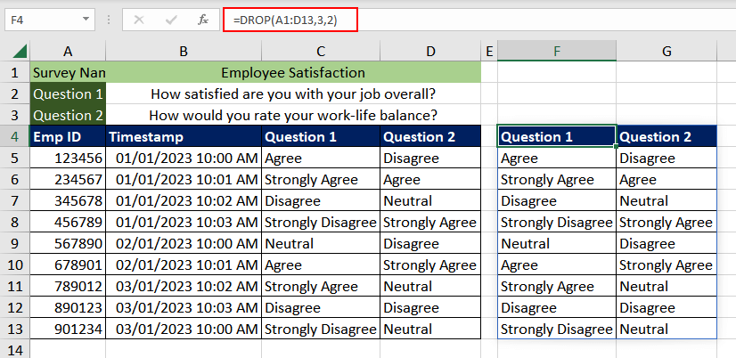
The new dataset can now be used to analyze employee satisfaction.

Example 2 – Removing Last N Rows or Columns using DROP Function

Suppose, we are planning to invest in a particular stock, and we download the daily stock prices of a company from the internet. The dataset includes information such as the date, the opening price, the closing price, the high and low prices, the volume traded, and other information.

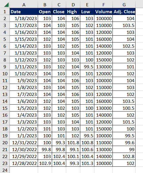
For better analysis, we wish to only focus on recent data. Also, columns containing information about  "volume traded" and "adjusted closing price" are irrelevant to us. Using the DROP function, we can exclude the last few rows containing data from last month and the last two columns from the given data.

As the DROP function counts rows and columns to remove from the starting of the array, we will use negative values for the rows and columns argument so that it counts from the end. The formula used will be as follows.

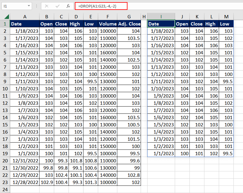
By cleaning up the data in this way, we can focus on the most relevant information and make more informed decisions based on recent trends. This was just an example with a smaller dataset. Try using the same logic when the existing dataset contains information from the past 10 years, but you only require 5 years.

Example 3 – Combining SORT and DROP Functions

In this scenario, we have received information about the annual sales of our global organization's stores in different countries. The data includes annual sales by each country, the highest performing month, and the number of employees for each country. Our goal is to find the top-performing countries in terms of annual sales.

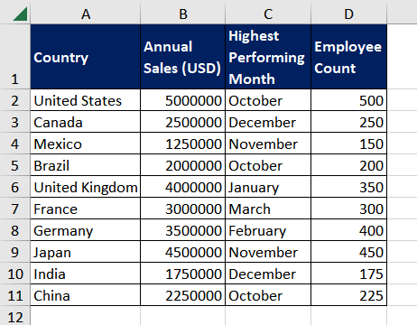
As we can see, the data is not arranged as per total sales. In order to exclude the countries with low sales, we will first have to use the SORT function to arrange the dataset by annual sales in descending order. To further clean the data, we can also remove the "Highest Performing Month" and "Employee Count" columns from the dataset as they are not relevant in this case.

To organise the data in descending order based on the second column containing the annual sales figures, the formula used will be as follows.

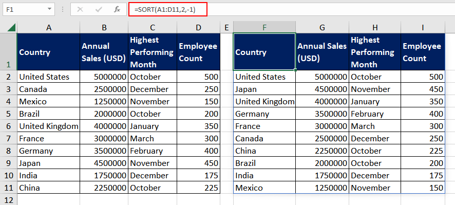
Once the data is sorted, we can use the DROP function to remove the last N rows and the last 2 columns from the data. The value of N depends on how many top-performing countries we want to keep. If we wish to keep the top 3 countries, we can remove the last 7 rows. The formula used will be as follows.

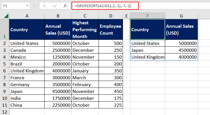
While we were able to easily count the number of rows to be removed in this particular dataset, this approach may not be ideal in cases where the dataset is much larger. To resolve that, we can use the ROWS function.

To improve the dataset, we will take a cell, say H1, where the user can enter the value of N, which is the number of top-performing countries we wish to retain in the dataset. We will then use the ROWS function to count the total number of rows in the range and then subtract the header row and the value of N (number of top rows to be retained). This will give us the number of bottom rows that must be removed.

The formula used will be as follows.

We can use this in the previous formula along with a minus sign. The updated version looks as follows.

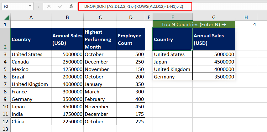
So, now no matter how the original dataset is arranged, you can easily sort and drop the data as per your requirement.

Example 4 – Combining Ranges and Dropping Rows or Columns

Assume that we run a small business and the dataset contains information about customer orders from multiple channels, such as online, in-store, and phone orders. Each channel has its separate dataset. For data analysis, we wish to remove all cancelled orders from the database.

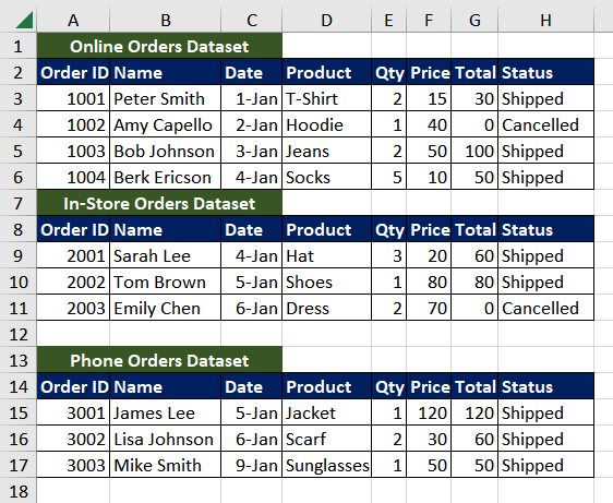
As they are in different datasets, we will have to use the DROP function separately. Instead, we can use the VSTACK function to combine all the datasets vertically into one. We can then use the SORT function to sort the 'Cancelled' orders. Finally, we can use the DROP function to remove the required rows and columns.

To combine all the datasets into one, the formula used will be as follows.

As all the cancelled orders have 0 as the 'total' value, we can use the SORT function to arrange the 7th column in ascending order. All the cancelled orders containing 0 as the Total value will be on the top of the dataset. The formula used will be as follows.

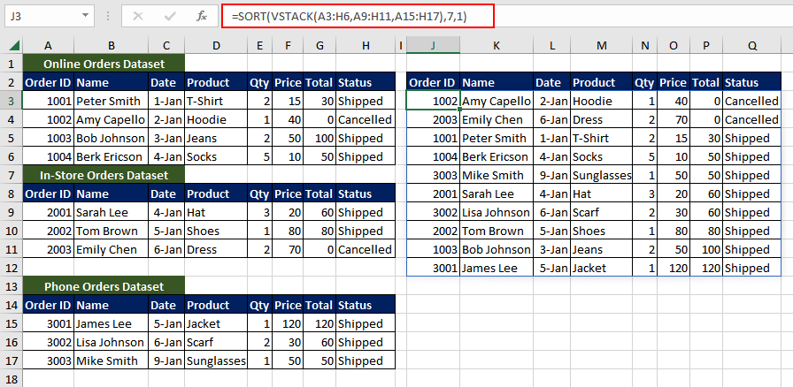
Finally, we use the DROP function to exclude the first two rows. To further clean the data, we can also remove the last column, as the dataset only contains 'Shipped' items. The final formula used will be as follows.

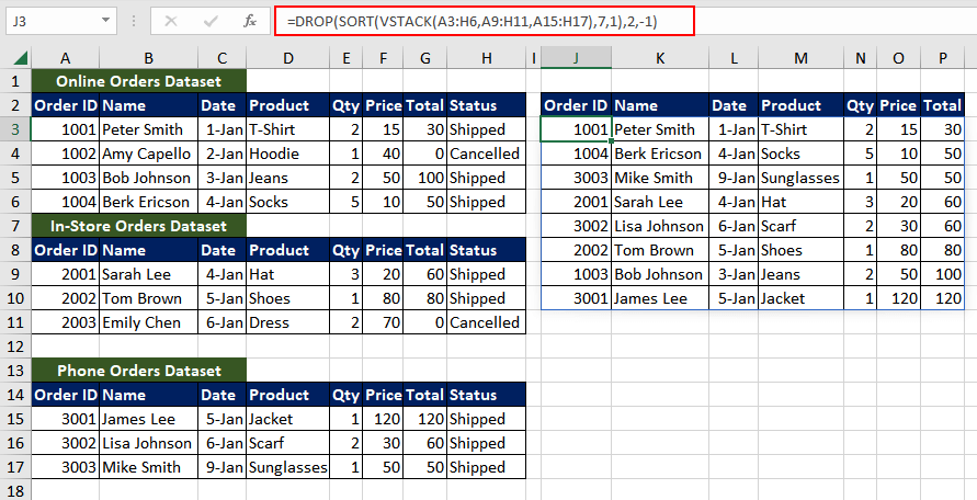
We can use the same logic with the HSTACK function, where we combine the datasets horizontally and then drop the irrelevant rows and columns as per the requirement.

DROP Function vs TAKE Function

Both DROP and TAKE functions are used to clean and manipulate data as per our requirements. Now we know that the DROP function removes the given number of rows and columns from an array, the TAKE function does the opposite.

The TAKE function extracts and returns the specified number of rows and columns. Let's understand it better with an example.

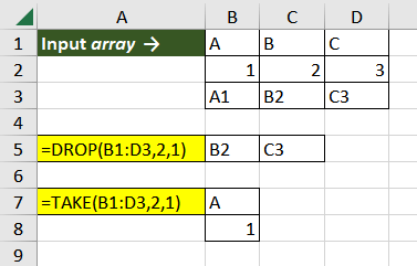
Here, we have taken a sample array with the range B1:D3, and the value of the rows and columns argument is 2 and 1. The formulas used are as follows.

As we can see from the resulting arrays, the DROP function removed the first two rows along with the first columns and returned the remaining array. On the other hand, the TAKE function kept the first two rows with the first column and removed everything else.

Now that the DROP function is a valuable addition to your Excel arsenal, find more ways to use it. It will drastically improve data analysis and manipulation and will speed up the process. We will soon be back with another valuable Excel function.