The Excel ERROR.TYPE function returns a number that corresponds to an error type. As the name suggests, the function only works for errors. Upon finding anything other than errors, the function returns the #N/A (not available) error. When an error is found, the function returns an integer (error code) that tells you the type of error.
But wait, what's the purpose of displaying a number instead of the error itself?
This is done so as to give the user an option to selectively handle one or more error types while ignoring other results. It allows us to have more granular control in error handling.

The ERROR.TYPE function was introduced in Excel 2003. Let's move onto its syntax.
Syntax
The syntax of the ERROR.TYPE function is as follows:
=ERROR.TYPE(error_val)Arguments:
'error_val '– The error for which the corresponding number would be returned.
The error codes returned by the Error.Type function are as follows:
| Error Code | Error Type | Error Name | Description |
|---|---|---|---|
| 1 | #NULL! | Null error | #NULL! error in excel is mostly because of typos, where a space character (' ') is incorrectly used in place of a colon (':') or comma (',') between two cell references. This happens because space character in excel corresponds to range intersect operator and by throwing #NULL! Error excel suggests that the supplied ranges do not intersect. |
| 2 | #DIV/0! | Divide by zero error | The #DIV/0! error indicates that the formula has been asked to divide a number by zero or a value that is equivalent to zero (like an empty cell). |
| 3 | #VALUE! | Value error | The #VALUE error is encountered when a value is not of the expected data type. It's Excel's way of saying there are incompatible data types in your expression or formula. |
| 4 | #REF! | Reference error | The #REF error means that a reference used in a formula has expired or invalidated. Most commonly, this is the case when a formula points to a cell reference that does not exist (for example, you deleted a row or a column that was being referenced by a formula). |
| 5 | #NAME? | Name error | The #NAME? error means that Excel is not able to recognize a formula name or some text used within the formula. |
| 6 | #NUM! | Number error | The #NUM! error signifies invalid numeric values in a formula or in the result of the formula. |
| 7 | #N/A | Not available error | This error indicates that a formula hasn't been able to find what it's set to look for. It is also triggered by an extra space between characters, incorrect spellings, or inconclusive lookup tables. |
| 8 | #GETTING_DATA | Getting data | #GETTING_DATA is actually not an error but a message that can show up when a large or complex worksheet is being calculated. While the calculations are still processing, the unfinished cells may temporarily display #GETTING_DATA message. |
| 9 | #SPILL! | Spill error | #SPILL ERROR occurs when a formula needs to return multiple results but is not able to return them to the grid because it is being obstructed by something on the grid. |
| 12 | #UNKNOWN! | Unknown error | The #UNKNOWN! error is caused by an unknown data type that is unsupported by the particular version of Excel in use. |
| 13 | #FIELD! | Field error | #FIELD error occurs in case of Linked or Rich Data Types. It arises when the record is insufficient to provide the relevant data for a referenced field. |
| 14 | #CALC! | Calculation error | #CALC error occurs when Excel's calculation engine runs into an unspecified calculation error with an array. |
Important Characteristics of ERROR.TYPE Function
- The function deals with errors only and in case of an error, the result will be a number that signifies the corresponding error.
- When no error is detected, the function returns an #N/A error.
- The function can be used along with the IF function for a custom text result.
Examples of ERROR.TYPE Function
What can this function do? Let's see with some examples.
Example 1 – Simple ERROR.TYPE function
Let's show you what the results look like when the ERROR.TYPE function is applied in its most elementary form.
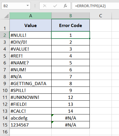
We are checking column A for errors using the formula super simply:
=ERROR.TYPE(A2)Here, the ERROR.TYPE function finds an error in "A2". The corresponding error code assigned by Excel to the #NULL! error is "1", which is the result in the first instance. Similarly, cells A3 to A14 also contain errors and hence the function returns their corresponding error codes.
Since the function only supports errors so it returns #N/A error for cells A14 and A15 as they contain text and numbers.
Example 2 – ERROR.TYPE function with IF function
Now, let's see an example where we only wish to handle #DIV/0! errors. When a #DIV/0! is encountered, instead of returning the error, we want to return a text saying "DIV BY ZERO ERROR!" for all other values or errors we want them to be displayed as it is.
Since, in this case, our objective is to handle a particular type of error so other error handling functions like IFERROR, ISERR, IFNA cannot be used. To accomplish this we will make use of the ERROR.TYPE function along with the IF function.
Let's see how:
=IF(ERROR.TYPE(A2) = 2,"DIV BY ZERO ERROR!",A2)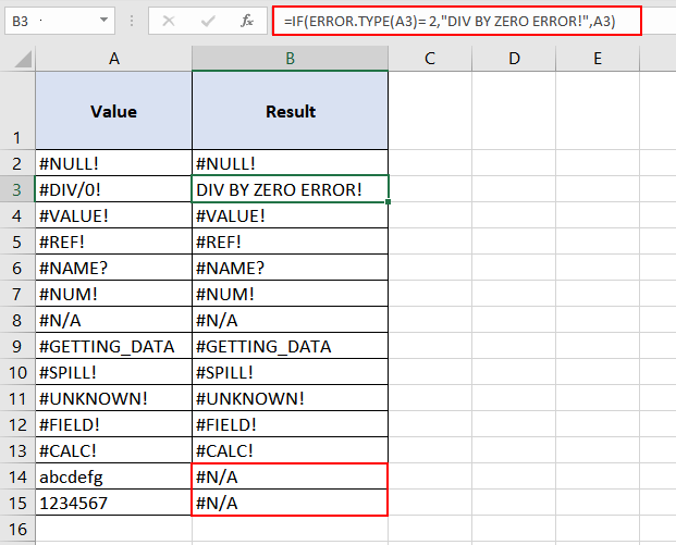
Here, in the above formula, we simply have examined cell A2 with ERROR.TYPE function and using the IF function, we are trying the find out if the result of ERROR.TYPE function is 2 or not.
Why 2?
Because 2 is the error code corresponding to the #DIV/0! error. If the ERROR.TYPE function returns 2, then we know it's a #DIV/0! error, and so we are displaying the relevant text message otherwise, the value of A2 is displayed.
Does it look perfect?
No, we have a problem here. If you look at cells B14 and B15 closely, you will see that they are now throwing a #N/A error.
Why did this happen?
To understand this, let's take a step back to see how the ERROR.TYPE function works. The first and foremost thing we need to do is realize a fundamental attribute of the ERROR.TYPE function – it returns a #N/A error when a non-error value or expression is passed to it.
Since the cells at A14 and A15 do not have errors, so the ERROR.TYPE function returns a #N/A error to the IF function, and since the IF function on its own is not able to handle this error, so it returns the error as it is.
To solve this, the simplest method is to have nested IF conditions as follows –
=IF(ISNA(ERROR.TYPE(A2)), A2, IF(ERROR.TYPE(A2) = 2,"DIV BY ZERO ERROR!",A2))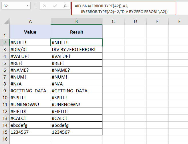
Here, first of all, using the ISNA function, we are trying to handle the #N/A errors thrown by the ERROR.TYPE function. If the ERROR.TYPE function throws a #N/A error; the ISNA function returns TRUE, and the outer IF function returns the value of A2 as it is. However, if the result of the ISNA function is FALSE, then there is another IF function (inner IF function) to handle this.
In such a case using the inner IF function, we examine if the ERROR.TYPE function returns 2 or not. If the ERROR.TYPE function returns 2, then we know it's a #DIV/0! error, and we display the message "DIV BY ZERO ERROR!" otherwise, the value of A2 is displayed.
Simple, Isn't It?
Now let's take things to the next level.
Example 3 – ERROR.TYPE function with IF & LOOKUP functions
Now our objective is to show a custom error moniker against each type of error, and for non-error values, we need to show them as it is. Let's work on the same table as in the previous example.
Although we could write a formula for this one similar to Example 2, but such a formula is going to be very long and complicated. Since it will involve multiple IF functions nested within each other.
So here is another way to accomplish it.
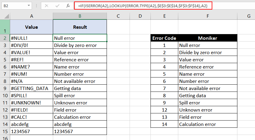
=IF(ISERROR(A2),LOOKUP(ERROR.TYPE(A2),$E$3:$E$14,$F$3:$F$14),A2)Here the ISERROR function checks A2 for an error and since A2 has an error so the ISERROR's result is TRUE. In case of TRUE, the IF function passes the result to the ERROR.TYPE and LOOKUP functions. The ERROR.TYPE generates the corresponding error code for cell A2. Next, the LOOKUP function fetches the relevant custom moniker from range E3:F14.
All the functions can take a deep breath now as that was the final outcome of the formula. In this way, the formula results in the respective text monikers for each error.
Let's assess an error-free cell. ISERROR checks A14 for errors since no errors are found; hence, the ISERROR function returns FALSE. In case of FALSE, the IF function displays the value at A14.
That's all! ERROR.TYPE has turned us down from saying more. We think it's becoming a habit.
How did the ERROR.TYPE function turn down the error-free cell?
.
.
.
"You're not my TYPE."
We will be back with more explanations from Excel functions!


