Excel EXACT Function – How To Use

The EXACT Function comes under the category of text functions in Excel. It is used to check two or more text strings, whether they are identical or not.

The EXACT function being a case-sensitive function compares both the text values and the character's case and then returns TRUE or FALSE.

Syntax

The syntax of the EXACT function is as follows.

Arguments:

The EXACT function accepts two mandatory arguments. The text arguments can be directly inserted in the function using double quotes or as cell references.

'text1' – The first text string that needs to be compared.
'text2' – The second text string to compare the first one with.

Important Characteristics of the EXACT function

The EXACT function is often compared with the standard equal to (=) operator, so the standout characteristic of the EXACT function is that it is case-sensitive. Other characteristics of the EXACT function are given below.

• The EXACT function ignores formatting.
• It is a logical function and returns TRUE or FALSE.

Examples of EXACT Function

We often have to compare two datasets in Excel for analysis or accuracy. One of the best ways to do so is using the EXACT function. Let's check the basic functionality of the EXACT function.

Here we are comparing two columns to check if they are identical.

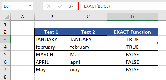
Using the formula as follows:

The EXACT function checked both the text strings, returning TRUE and FALSE. As observed, In the first case since both of the strings are in uppercase so the function returns TRUE. Similarly in the second case since both the strings are in lowercase, so the function again returns TRUE.

In the third case, both the strings are different hence the function returns FALSE. In the fourth and fifth case even though the content is identical, but the letter case varies. Hence, we get FALSE from the EXACT function.

Example 1: Comparing Two Lists of Data

In this example, we have a dataset with some famous TikTok account names and usernames. We also downloaded a list of famous TikTokers worldwide and would like to compare if both lists match.

Assuming that the usernames are case-sensitive, we will use the EXACT function to compare the two lists. Using the formula as follows:

The first username in cells C3 & D3 is an exact match, whereas cells C4 & D4 are different because a few letters in cell D4 are in uppercase. The same is the case with the 3rd and 4th usernames.

Example 2: Using EXACT Function with Dates

Now that we have understood the functionality of the EXACT function with text, what if the dates are written in different formats? Will the EXACT function return TRUE or FALSE? Let's find out.

Here, we have one date written in different formats. The first two are different formats of dates in Excel, whereas the third format is the general format. In Excel, dates are stored as numbers, and what we see is actually a format.

We will use the EXACT function to compare the three formats with each other. The formula used will be as follows.

The EXACT function has been used to compare B3 with C3 and then with D3, and C3 with D3. Even though all the dates look different, as per the EXACT function, they are all identical, therefore, despite being case-sensitive, the EXACT function ignores formatting variations and returns TRUE for all three comparisons.

Example 3: Finding Exact Match from a List

By now, we have understood how to compare two values. We might need to search for an exact match in a list of values rather than merely comparing one cell to another. One of the best applications of this logic is to check product availability in our database using product codes.

The product codes depending on nomenclature and company standards might be case-sensitive. So, here we have a set of codes with their associated products.

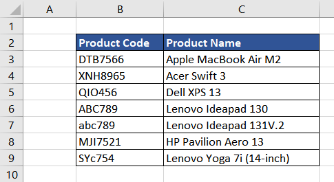
We wish to check if the required product code is available in stock. We could quickly do a CTRL+F, but it is not an efficient solution when used on a bigger dataset. Instead, we let the user enter the product code and check for its exact match.

The formula used will be as follows.

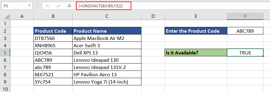
We can enter the code of the product that we are looking for in cell F2. We then use the EXACT function comparing F2 with the complete list of product codes which in this case is from cell B3 to B9. Then, we wrap the complete function in OR function to ensure that any match results in TRUE. As the final bit, press the Ctrl + Shift + Enter keys to add curly brackets and make an array formula.

The OR function returns TRUE if any of the conditions is true and returns FALSE when all the logical conditions are false. Without the OR function and conversion of the formula, the EXACT function will return TRUE or FALSE for each comparison which is not ideal.

An array formula will calculate each result in the range B3:B9 as FALSE, FALSE, FALSE, TRUE, FALSE, FALSE, FALSE. The OR function returns TRUE upon finding even one TRUE instance and has therefore been confirmed that ABC789 is available.

In another scenario, you can use the AND function in an array formula if you want TRUE to only be returned when all the conditions are met.

Example 4: Using EXACT Function in Data Validation

We can also use the EXACT function to ensure that any data entered in the sheet is in the desired format. For example, in the guest book, the names entered must be in the proper case, i.e., the first and the last name must begin with a capital letter.

This way, the data collected will be in the format we want. Using the Data Validation option in Excel, we can choose a custom setting and use the EXACT function to our advantage.

Select the cells where you want to apply Data Validation. Under the Data tab, choose Data Validation.

Under the Settings tab, choose Custom from the Allow option. In the Formula tab, enter the Excel formula as follows.

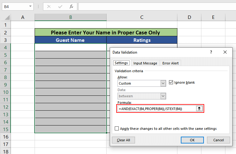
Press OK and you are all set.

Now, let's understand the Excel formula we used.

When a user adds or modifies a cell value, the Data Validation rules we specified will be activated. The PROPER function converts the input value into the proper case (capital initial). Then, the EXACT function conducts a case-sensitive comparison. So, till now the Excel formula is as follows.

The ISTEXT function checks whether the value entered by the user in B3 is text.

Now, put both logical conditions in the AND function. The AND function returns TRUE only if both the conditions are true, else the input value fails the Data Validation.

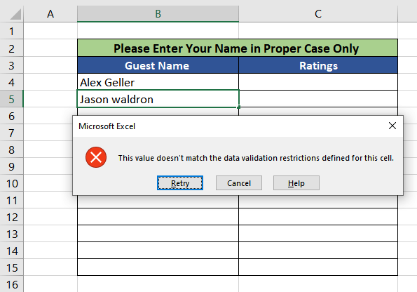
The following error will appear for any input value that is not in the proper case or is not a text value.

Example 5: Counting Case-Sensitive Repetition

Suppose we have received a list of Instagram influencers to use for our next marketing campaign. To verify how often they post, we downloaded the data, which contains their account names, and every time they post on the social media platform with dates.

We can simply count the number of times a username is repeated to get the total number of posts in the same time period. We are also assuming here that the usernames are case-sensitive.

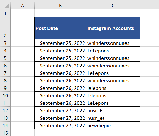
Excel functions like COUNTIF and COUNTIFS can be used, but they are not case-sensitive functions. To count the repetition in a case-sensitive manner, we will use a combination of SUMPRODUCT and EXACT.

The EXACT function will compare each unique username to the complete data in column C. The double negative or double unary will then convert TRUE and FALSE into 1s and 0s. Finally, the SUMPRODUCT formula will have a series of 1s and 0s to add and give us the final value, which is the number of times the user posted under the unique username.

Let's decode every step in terms of return value to understand it better. We will explain the function inside out.

The EXACT function compares the value of each unique username in cell E3 to all values in C3 (kindly fix this in the formula in the following screenshot) to C14. As we provided multiple values in the second argument of the EXACT function, it returns multiple results. In this case, the EXACT function returns 12 values in an array in the form of TRUE and FALSE.

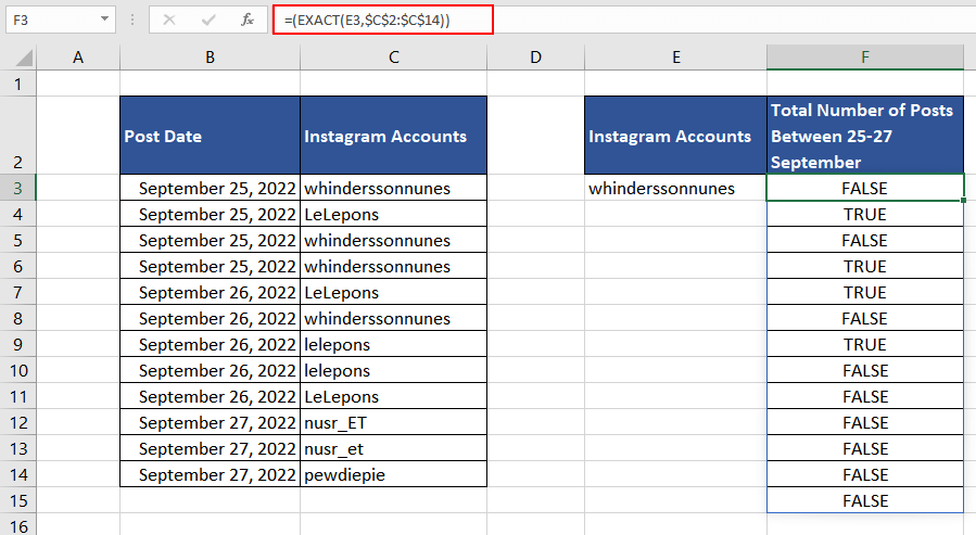
As explained earlier, the EXACT function returns a series of TRUE and FALSE. The double negative converts all the TRUE & FALSE into 1s and 0s.

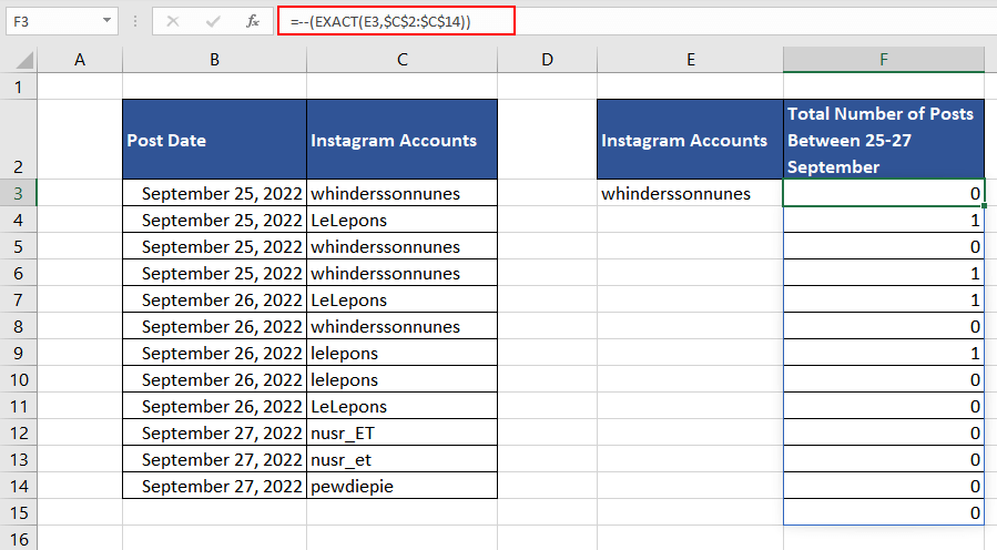
The final step is combining everything into the SUMPRODUCT function, which will give us the sum of the array. Also, we added a dollar sign with the range C2:C14 as we want it as an absolute cell reference. The final formula will be as follows.

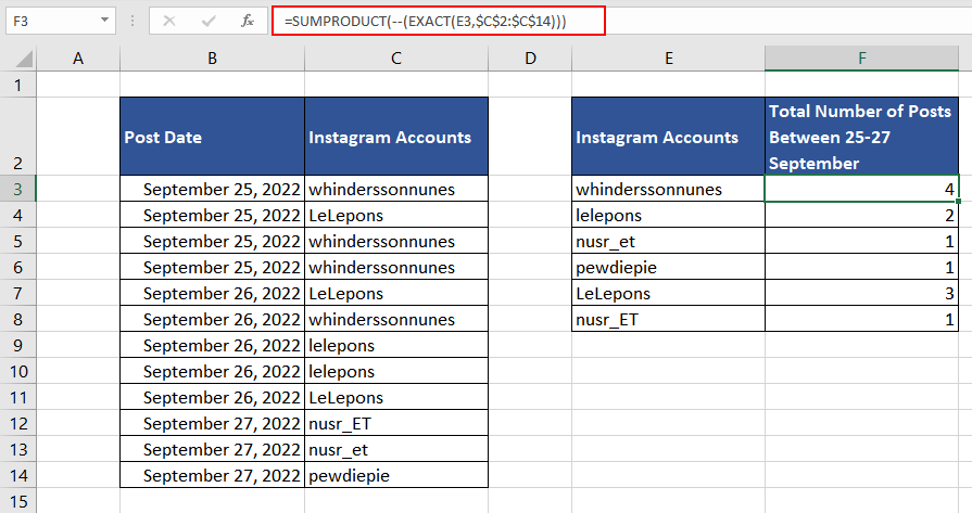
We can also use the SUMPRODUCT and EXACT functions for case-sensitive lookup.

Example 6: Counting Sum for Exact Matches

Suppose after calculating the frequency of content posted by each influencer, we had to calculate the total number of likes and comments they get. It will be easier to decide on the one to pick.

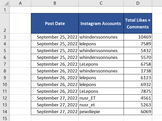
We can use an Excel function like SUMIF, but it is not case-sensitive. With the help of EXACT and SUMPRODUCT functions, we can calculate the sum of total likes and comments for each unique username.

The formula used will be as follows.

Similar to the above example, the EXACT function will compare each unique username in cell F3 with all the usernames in column C. The return values will be TRUE or FALSE.

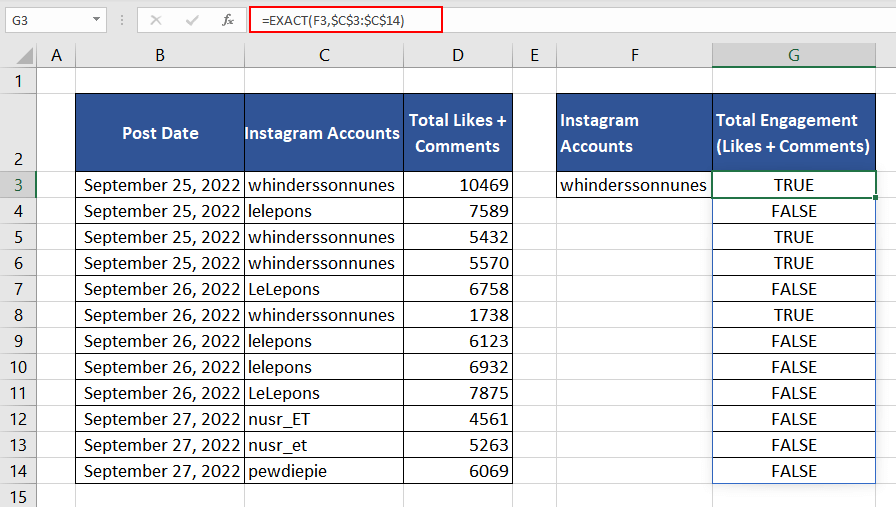
To remove the need to use a double negative operator, we will use the mathematical operation of multiplication (*), which converts TRUE and FALSE values to 1s and 0s. Any false value will be 0 due to the multiplication.

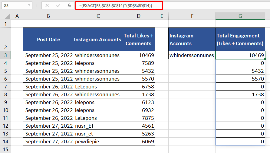
Finally, the SUMPRODUCT of all the match results will give us the final case-sensitive lookup addition.

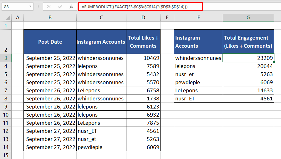
Note: The only limitation of this case-sensitive lookup is that it cannot return text values, as the multiplication function cannot be performed. To look up a case-sensitive exact match and its corresponding text values, we can use the INDEX or MATCH function in combination with the EXACT function.

Using Equals Operator vs EXACT Function

The equals sign (=), when used with two variables, acts as a comparison operator. The only difference between the equals sign and the EXACT function is that the EXACT function is case-sensitive, where as equals operator is not case-sensitive.

Lets get back to our initial example and compare the results of EXACT function with Equals operator.

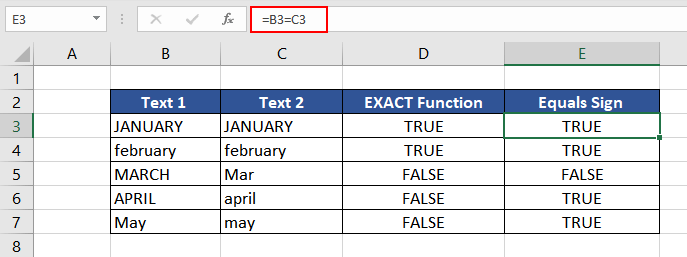
You would observe that the Equals operator returns TRUE in all the cases except the third one. In third case, the text strings to be compared are different and hence both the Equals operator and the EXACT function return FALSE.

For all the other cases, Equals operator returns true since the text strings are same.

In a nutshell, the equals operator checks text values, whereas the EXACT function checks both the text values and the text case.  In the case of numeric values, dates, or time, both return similar results.

We're through with the EXACT function, but we promise not to take too long before coming back with another function that you can add to your Excel toolkit.  Practice and explore more interesting ways to use the EXACT function.