Excel ISERR Function – How to Use

The Excel ISERR function checks whether a value is an error (except for the #N/A error) or not. The function returns TRUE upon finding any error except the #N/A. It returns FALSE for all other values and for #N/A errors.

ISERR literally means ‘Is error?’, but by shortening the spelling, it hints that it would not work for #N/A errors. This may seem like a shortfall but there are functions that deal with all types of errors and few other functions that singularly deal with the #N/A errors. With its introduction in 2003, ISERR comes from a bunch of IS functions that result in TRUE or FALSE.

By the end of this tutorial, you will learn what the ISERR function can do, how to increase its usefulness with other functions, and how it stacks up against similar error handling functions.

Syntax

The syntax of the ISERR function (like all IS functions) is as follows:

Arguments:

value – The value or expression to be tested for errors (except for #N/A error).

Important Characteristics of ISERR Function in Excel

• The ISERR function deals with all errors except #N/A errors.
• The function returns TRUE when it finds errors other than the #N/A error, otherwise, it returns FALSE.
• ISERR is generally used along with the IF function to handle errors.
• If the formula has any typos or misspelling, the function returns a #NAME? error

Examples of ISERR Function

Let’s look into some examples to increase our understanding of the ISERR function.

Example 1 – Simple ISERR function

Let’s see ISERR in its simplest form to show you what it can deal with.

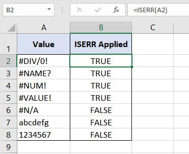
We are checking column A for errors using the ISERR function in its simplest form:

Here, the ISERR function looks for any errors in cell "A2" and since cell "A2" has a #DIV/0! error so the function returns TRUE. In addition to "A2", all the cells from "A3" to "A5" also contain errors hence the ISERR function returns TRUE for all of them.

However, upon finding an #N/A error in the cell "A6", ISERR results in FALSE. Similarly, it also results in FALSE upon finding no errors in cells "A7" and "A8". This confirms that the ISERR function picks on all errors except #N/A errors.

This is a very basic application of the ISERR function. Let’s see more practical examples.

Example 2 – ISERR function with IF function

The easiest way to expand the usability of IS family functions is to nest them within the Excel IF function. The IF function delivers custom values for when a supplied condition is met or not. We can achieve these custom values instead of TRUE/FALSE by using the IF and ISERR functions together. Let's see this with an example.

We have a list of 10 products. We are given the total sales for each product and its unit price. We are calculating the units sold of each product ( dividing sales by price).

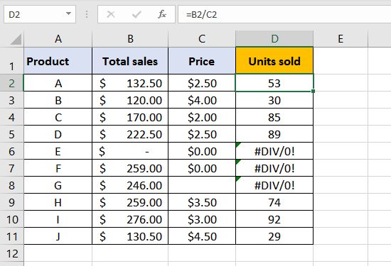
The absence of the price of some products has resulted in #DIV/0 errors. We are not liking the look of these on our worksheet so let’s use the said functions to present the errors in a more elegant way.

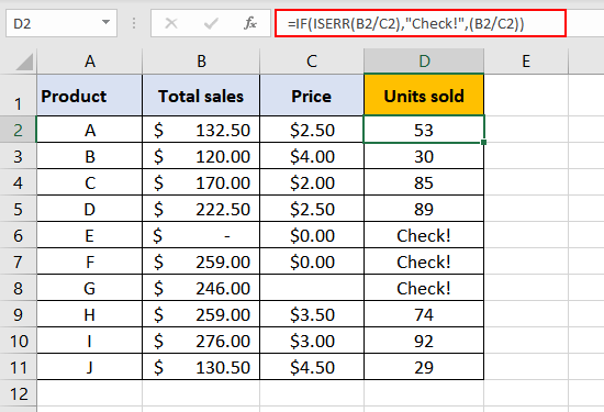
We have converted the #DIV/0 errors into the custom value "Check!" by this formula:

The purpose is to check errors while calculating units sold and attain a custom value instead of a #DIV/0 error.

Beginning with Product A, the ISERR function starts off by checking "B2/C2″ for errors. It finds no errors, ISERR’s result is FALSE. In case of FALSE, the IF function is set to deliver the result of “B2/C2" (which is 133/2.5). The result is "53" which is finally displayed.

Let’s evaluate the #DIV/0 errors. Product E hasn’t been launched yet, hasn’t made any sales and so its data is not available. ISERR checks "B6/C6" for errors, it finds a #DIV/0 error (0/0 = #DIV/0), ISERR’s result is TRUE. In case of TRUE, the IF function is set to deliver the result "Check!", instead of displaying the #DIV/0 error, which is the final result.

We can also see the same treatment for Products F and G. Product F’s sales data is available but the price is listed as $0 which results in a #DIV/0 error. Product G’s sales data is available but the price data is missing which again results in a #DIV/0 error. The IF function has displayed both the #DIV/0 errors as the custom value "Check!".

Example 3 – ISERR function with the SUM function

The SUM function adds all the numbers in the provided range of cells. We can take the help of the SUM and ISERR functions to count how many errors (except #N/A errors) there are in a range of cells supplied in the formula.

We will take a look at Example 1.

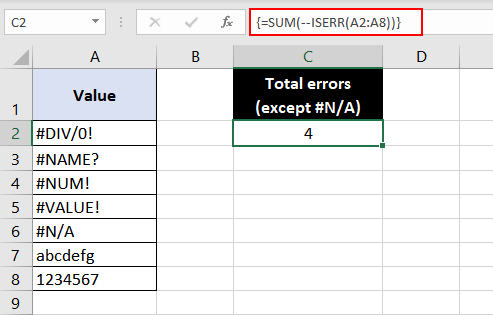
The formula used is:

Note: This is an array formula and must be entered with Ctrl + Shift + Enter keys, except in Excel 365.

The ISERR function applied to the range on its own will split into the supplied cell range and give the result of each cell individually in this way:

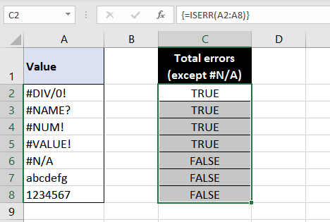
The #N/A error is excluded from being treated as an error by the ISERR function. The result of the ISERR function is TRUE, TRUE, TRUE, TRUE, FALSE, FALSE, FALSE. The double unary in the formula commands TRUE and FALSE to take their respective numeric values as 1 and 0. The result then becomes 1, 1, 1, 1, 0, 0, 0. The SUM function then adds up ISERR’s result and displays "4" as the result.

Where #N/A errors need to be included in the errors, the ISERROR function can be used instead of the ISERR function in the same way.

Recommended Reading: Excel IFERROR Function – How to Use

ISERR vs ISERROR Function

The bigger brother of ISERR, ISERROR (is error?) deals with all Excel errors and returns TRUE if any error is detected and FALSE otherwise. Unlike ISERR, ISERROR accounts for the #N/A error along with other errors.

Let’s see what changes using ISERROR instead of ISERR can bring to the above example.

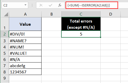
Without changing anything else, we have replaced the ISERR function with the ISERROR function in the formula:

Note: This is an array formula and must be entered with Ctrl + Shift + Enter keys, except in Excel 365.

The result here is "5" instead of "4" because the ISERROR formula returns TRUE for the #N/A error as well (unlike ISERR). The inner function results in – TRUE, TRUE, TRUE, TRUE, TRUE, FALSE, FALSE. The double negatives change result to 1, 1, 1, 1, 1, 0, 0. The SUM function then adds up these numbers to "5" and displays the final result.

How to Choose Between ISERR & ISERROR

The ISERR function is suitable where the #N/A error is not required to be accounted for as an error. Where the #N/A error needs to stand out without being covered as any other error, the ISERR function would be a good choice so as to point out that certain data is not available.

On the other hand, the ISERROR function would work better where all errors need to be handled.  It will deal with all errors including the #N/A error and will confirm whether there are any errors in the data or not.

Both functions result in either TRUE or FALSE and can use the IF function to return custom values instead of TRUE/FALSE.

ISERR vs ISNA Function

The ISNA function is the exact opposite of the ISERR function; the ISNA function checks whether a value is #N/A and returns TRUE or FALSE accordingly. For what the functions offer, they are both useful in their own regard and depend on what you are trying to achieve. Like in the example above, ISNA would be totally irrelevant as we are not dealing with #N/A errors which usually comes up alongside lookup functions.

Replacing ISERR with ISNA in Example 2 would do this:

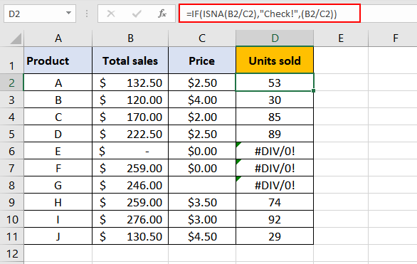
The ISNA function solely deals with #N/A errors and has resulted in #DIV/0! errors despite the request to return "Check!" upon finding errors. But let’s not judge a fish on its ability to climb a tree.

Now if we were to look up the units sold for certain products, this is what we would do:

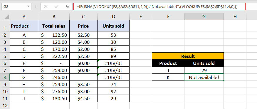
VLOOKUP is told to find the data in the cell "F8" which is Product "K". The table given to VLOOKUP for searching is within the cell range "A2:D11" (locked in place by the “$” sign); VLOOKUP must find the value in "F8" cell in the 1^st column (column A) of the given table and return the corresponding value from the 4^th column (column D). "0" indicates that VLOOKUP must find an exact match. However, VLOOKUP could not find Product "K" in column A as it is not listed in our dataset.

This results in an #N/A error. The result is handed over to ISNA and it turns "#N/A" into TRUE. The result TRUE is passed to the IF function which shows the message "Not available!" as the final output of the formula.

NOTE: Check out the IFNA function which will give identical results without having to nest the ISNA function within the IF function.

Replacing ISNA with ISERR in this example would do this:

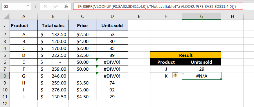
The ISERR function does not deal with #N/A errors and has resulted in an #N/A error as VLOOKUP could not find Product "K" in the dataset.

How to Choose Between ISERR & ISNA

When in need of narrowing down the errors to be checked, IFERR will work for covering up all errors excluding the #N/A error. It is the exact flip of the ISNA function which will be convenient to deal only with #N/A errors. Both result in TRUE/FALSE upon finding the respective errors and need IF to result in custom values. When dealing with all errors minus the #N/A error, use ISERR function.

The nature of the ISNA function is to exclusively deal with #N/A errors which makes it more useful with lookup functions and for such instances, ISERR becomes totally irrelevant. When ISNA will be used, it will only deal with #N/A errors and display other errors as is, which is helpful to find the underlying problem in the data or formula. When dealing only with #N/A errors, use ISNA function.

That’s practically the end but do you know how the shy guy asked out the new girl Isna on Excel?

.

.

.

.

.

IS, ERR, ISNA your #NAME?

We’ll be back with more functions and confidence!