The MATCH function in Excel is used to locate a specific value within a cell range or array. It gives us the relative position of the data we are looking for within the array or cell range.
The MATCH function proves especially invaluable when handling large datasets, as it enables swift and efficient identification of relative data locations, sparing the need to manually scour the entire dataset for the desired information.

Syntax
The syntax of the MATCH function contains three arguments out of which one is an optional argument.
=MATCH(lookup_value, lookup_array, [match_type])Arguments:
'lookup_value' – This is a mandatory argument that accepts the value we want to find within a given cell range or array. The input data in the lookup_value argument can be a number, text, or logical value. It can also be a cell reference containing the data.
'lookup_array ' – This is also a required argument as it contains the cell range or array in which we want to search for the lookup_value. The value of the lookup_array must be a one-dimensional array either vertical or horizontal. It is important to note that the lookup_array must be sorted in ascending or descending order for the MATCH function to work correctly with certain match_type.
'match_type' – This is an optional argument that determines which type of match we wish to perform. The acceptable input values for the argument are -1, 0, or 1 and when left empty, the default value for this argument is 1. When the value is set to 1, the MATCH function locates the largest value that is less than or equal to the lookup_value.
The lookup_array should be sorted in ascending order. If set to 0, it indicates that we are looking for an exact match. If it is set to -1, the function searches for the smallest value that is greater than or equal to the lookup_value. The lookup_array must be sorted in descending order.
Now that we know all the possibilities of using the above-mentioned arguments, let's look at a few characteristics of the MATCH function before we dive into some exciting applications and examples.
Important Characteristics of the MATCH Function
One of the most notable features of the MATCH function is that it is not case-sensitive. Some of the other aspects of the function that are noteworthy are as follows.
- When the MATCH function cannot locate the value, we are looking for, it returns a #N/A error.
- One limitation of the MATCH function is that it only works with text up to 255 characters in length.
- In case of a duplicate or more than one occurrence of the lookup_value in the data, the MATCH function returns the first match.
- When match_type is set to 0 and the data in the lookup_value argument is a text string, we can also use wildcard characters such as the question mark (?) and the asterisk (*). The question marks represent any single character while the asterisk is used to match any sequence of characters before or after. If you wish to locate an actual question mark or asterisk, simply precede it with a tilde (~).
Examples of MATCH Function
Let's begin with understanding all the arguments and how they contribute to the MATCH function. Here we will take a sample dataset and use different input values for each argument allowing us to gain deeper insights into the function's workings.
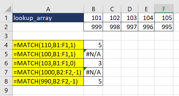
In the first two examples, the input value of the match_type is set to 1. In the first case, we are looking for the value '110' in the array B1:F1. As the lookup_value is not in the dataset and the match_type is set to 1, the MATCH formula looks for the largest value that is less than 110 in the array. As a result, the function returns 5 as the array is sorted in ascending order.
In the next instance, we are looking for the value '100' and the remaining argument values remain the same. As a result, the MATCH function returns a #N/A error as there is no value that is equal to or is less than 100.
The third example is an ideal case scenario, where we are looking for an exact match for the value '103' in the array. The MATCH function locates the same and returns the position of the lookup_value.
In the last two examples, we are exploring the behavior of the MATCH function where the value of the match_type is set to -1. In such scenarios, the MATCH function identifies the smallest value that is equal to or greater than the lookup_value. So, we can see that when we are looking for '1000', the function returns an error as there is no data bigger than 1000 in the dataset. On the other hand, when the lookup_value is 990, the MATCH function returns 5 for '995' which is the smallest value that is greater than '990'.
Example 1 – Simple Use of MATCH Function
Suppose you own a furniture store that sells various products such as bookcases, sofas, etc. You now have the dataset which contains details such as product IDs, product names, and total sales for each product to date.
You now wish to determine the ranking of the product based on their sales using the product IDs.
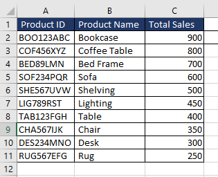
We can take cell E1 where the user can enter the product ID to look for. We can then use the MATCH function to determine the position or row number of the product ID. As we are looking for an exact match, the formula used will be as follows.
=MATCH(E1,A2:A11,0)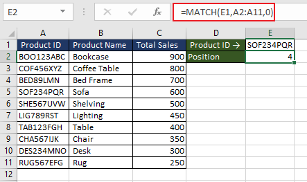
This is extremely useful when the dataset is large. As the current dataset is sorted from highest sales to lowest, the result obtained from the MATCH function also provides us with the product's ranking or popularity based on sales.
Furthermore, it is evident that the product IDs are crafted in a way where the initial three letters of the product ID align with the initial three letters of the product name. In case the user does not remember the entire product ID, we can take advantage of the wildcard characters supported by the MATCH function. Next, we'll show you how to do that.
Example 2 – Using Wildcard with MATCH Function
To simplify the user experience, we can ask them to just enter the initial three letters of the product name. Subsequently, we modify the lookup_value argument, where we combine the user-entered first three letters of the product with the wildcard character '*'. This means that the MATCH function will look for a value that begins with the user-entered text followed by any number of characters. The formula will be as follows.
=MATCH(E1&"*",A2:A11,0)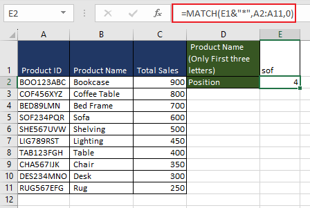
The asterisk has served as a buffer for the remaining characters of the product code "SOF234PQR" beyond the characters entered in E1. As observed in the previous example and stated in the characteristics, the MATCH function is case-insensitive. In the next example, let's explore the possibility of using the MATCH function in a case-sensitive manner.
Example 3 – Making MATCH Function Case-sensitive
Suppose you are a marketing manager planning a fresh marketing campaign for your company, and you wish to collaborate with social media influencers to promote the campaign. You have a dataset that includes details of potential influencers, such as their name, username, and the number of followers they have on social media.
To make it easy to filter out, you now wish to identify the position of the influencer based on their username.
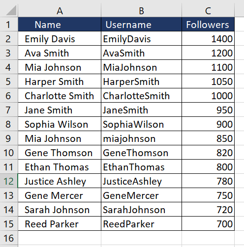
As we can see, the usernames contain both uppercase and lowercase letters, making it clear that relying solely on the MATCH function would be insufficient. Instead, we will use a combination of the EXACT function with the MATCH function.
The EXACT function will search for an exact case-sensitive match of the lookup_value. If it finds a match, the EXACT function returns TRUE, else it returns FALSE. The formula used will be as follows.
=EXACT(E1,B2:B15)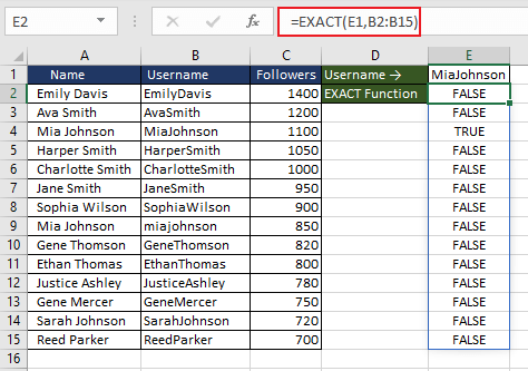
The EXACT function returned an array of TRUE and FALSE indicating where it found a perfect case-sensitive match. Now, we can use the MATCH function to look for "TRUE" in the previous array. The formula used will be as follows.
=MATCH(TRUE,EXACT(E1,B2:B15),0)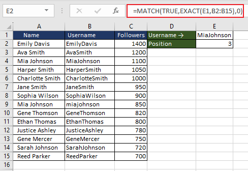
So, together, the EXACT function helps us figure out if there is a perfect match, and the MATCH function helps us find where that perfect match is in a list.
There have likely been multiple occasions when you've had to compare two columns to determine matches and differences. Employing the MATCH function is one effective method for accomplishing this task. Let's learn how to use it in the next example.
Example 4 – Comparing Two Lists Using MATCH Function
In this scenario, we have an upcoming technical training program that is open to all teams in the company. We now have two lists of email addresses, the first list contains the email addresses of the technical team, and List 2 contains a list of email addresses of employees who have been invited to a special training program.
The goal is to determine which email addresses from the training program list are a part of the tech team and which ones are not.
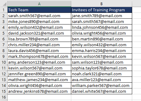
First, the MATCH function compares each cell in column B with all the data in column A. The formula used is as follows.
=MATCH(B2,A:A,0)We drag and drop the formula till the end of the dataset.
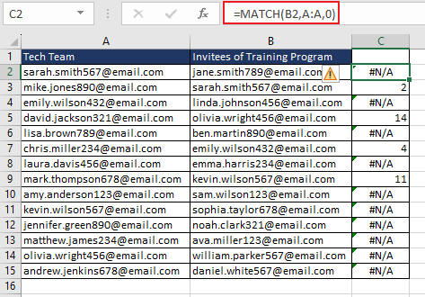
The next step is to check if the return value of the MATCH function is an error (specifically, a #N/A error). If there is an error, the ISNA function returns TRUE; otherwise, it returns FALSE. The formula will be as follows.
=ISNA(MATCH(B2,A:A,0))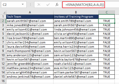
The last step is the simplest where we enclose the above formula in a basic IF function. It checks the return value of the ISNA and MATCH functions. If the value is TRUE, meaning the email address in column B was not found in column A), it displays "Not in Tech Team"; otherwise, it displays "Member of the Tech Team." The complete formula will be as follows.
=IF(ISNA(MATCH(B2,A:A,0)), "Not in Tech Team", "Member of the Tech Team")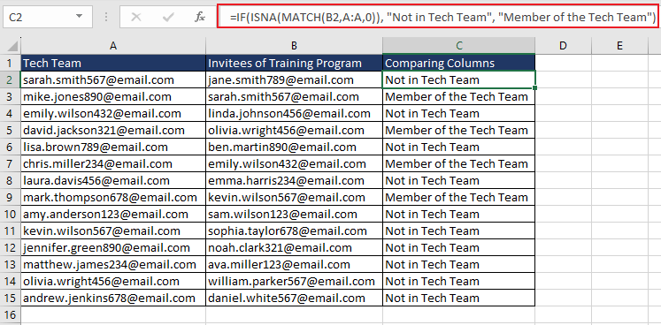
In case, the columns to be compared contain case-sensitive values, combine the logic mentioned in the previous example to improve this formula.
Example 5 – Using VLOOKUP with MATCH Function
Suppose you work in the HR department, and you have an Excel dataset containing information about employees, including their names, departments, and salaries. Now, you want to retrieve an employee's salary based on their name.
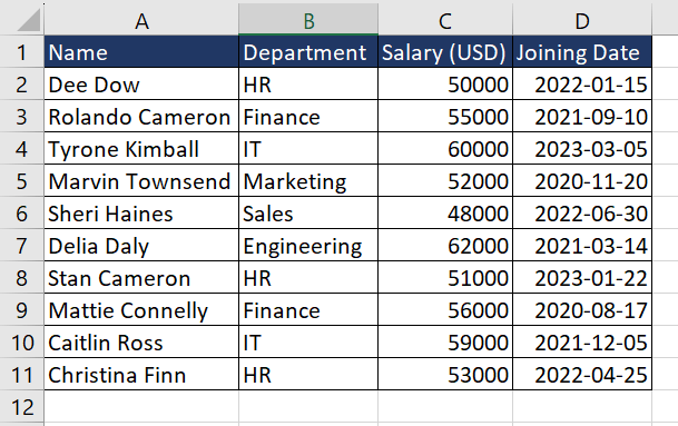
The easiest and the most preferred option is to use the VLOOKUP function. The formula used will be as follows.
=VLOOKUP(G1,$A$2:$D$11,3,FALSE)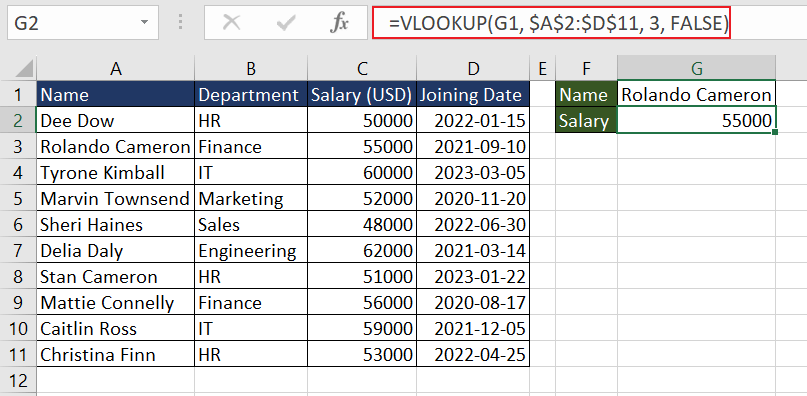
Problem solved. Now, due to some reasons, you had to delete Column B containing the details about 'Department'. Upon deleting the column, the above formula adjusted the value of the table_array but returned the value from the third column, which is 'Joining Date'.
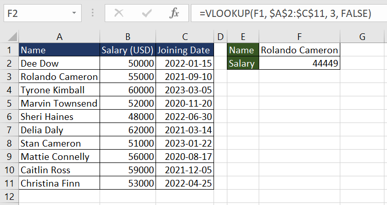
This is a limitation of the VLOOKUP formula where if we add or delete columns, the function returns incorrect data. In this case, if we delete column C as well, the function will return a #REF! error. To avoid this issue, we can use the MATCH function to dynamically determine the column index for the VLOOKUP function.
For instance, in this example, we are looking for values in the column named 'Salary (USD)'. Using the MATCH function, we can dynamically determine the column index by finding the position of "Salary (USD)" in the first row (row 1) of the data. This ensures that if we add or remove columns, the formula will still work correctly. To find the column number, the formula used will be as follows.
=MATCH("Salary (USD)",A1:D1,0)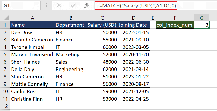
Now, we can use this in the above-mentioned VLOOKUP function. The formula will be as follows.
=VLOOKUP(G1, $A$1:$D$1, MATCH("Salary (USD)",A1:D1,0), FALSE)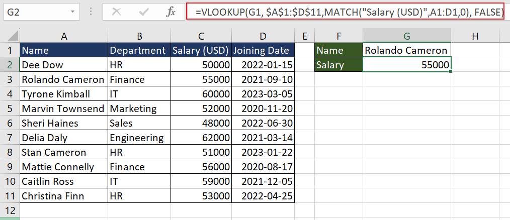
Now, even if we add or delete columns in the data table, the formula will still correctly retrieve the salary because it uses the MATCH function to determine the column index dynamically based on the column header 'Salary (USD)'. The same logic can be applied while using the HLOOKUP function.
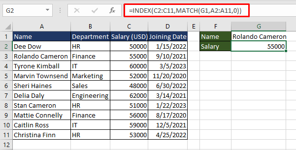
Alternatively, we can fix the column again using the MATCH function but use the INDEX function to return the match against the lookup value. The MATCH and INDEX functions are often used as a duo and now you'll see why. Use the formula below as a base to retrieve data relevant to the lookup value without facing trouble from dynamic changes:
=INDEX(C2:C11,MATCH(G1,A2:A11,0))Since the functions aren't restricted to retrieving data from the 3rd column, the result won't be subject to fluctuations with changes in the dataset. The MATCH function locates an exact match of the value in G1 in A2:A11 as 2. The INDEX function takes that position and returns the corresponding value from C2:C11 which is 55000.
Practice more yourself to discover how the MATCH function fits into your work and projects. While you uncover more exciting applications, we will work on yet another Excel function to add to your repository. Stay tuned for an even broader range of Excel tools at your fingertips.


