The MID function returns a specific number of characters from the middle of the string after we state the starting position and the number of characters to extract. The MID Function in Excel is one of the text functions that allows us to get a substring from a string\text as per our requirement
It is one of the most useful functions when we want to extract the middle name from the full name, the domain name from email IDs, or any substring between two characters.

Syntax
The syntax of the MID function is as follows:
=MID(text,start_num,num_chars)The MID function in Excel accepts three arguments and all three arguments are mandatory.
Arguments:
'text' – This holds the value of the input text/string. A cell reference containing the input string or text enclosed in double quotes are both acceptable input values.
'start_num' – The position of the first character we want to extract. It must be an integer/formula which indicates the starting position of the extraction.
'num_chars' – Number of characters we wish to extract from the starting point. The num_chars argument indicates the character length of the return value.
Important Characteristics of the MID Function
One of the essential and basic characteristics of the MID function being a text function is that it always returns a text value regardless of the input value. Even if the retrieved substring is only made up of numbers, it will be in text format. Other important MID function features are as follows:
- If the value of start_num exceeds the length of input text, the MID function returns "" (empty text).
- If the start_num value is less than 1, the function returns a #VALUE! error.
- If the value of num_chars is a negative number, the MID function gives a #VALUE error.
- If the num_chars value is less than 1, then the MID function's return value is an empty string, a blank cell.
Last of all, if the sum of the value of start_num and num_chars is greater than the total input text length, the MID function returns all the characters from start_num to the last character. This characteristic comes in very handy for certain conditions. We will find out in the examples below.
Examples of MID Function
The MID function can be used independently or can be combined with various other Excel functions such as SEARCH, FIND, LEN, and more. Let's go through some examples to fully comprehend the usage and utility of the MID function.
Example 1: Basic Functionality of the MID Function
In the below example, we have taken 3 different instances and tried using the basic MID function.
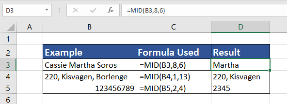
In the first case, the input text/string is a full name 'Cassie Martha Soros' where we wish to extract the middle name –"Martha". So, using the MID function we apply the formula:
=MID(B3,8,6)Here, the first parameter text is the cell reference B3. The second parameter start_num is the starting position which is 8 as the first name is 6 characters long, the space is the 7th character and then we add 1 so that we reach the beginning of the middle name. Lastly, the third argument num_chars is the number of characters of the middle name which is 6.
The second instance is where we are trying to extract the house number and street address from the complete address in cell B4. We are checking if the MID function counts a special character (,) and also whether the MID function can return characters from the beginning of the text or only from the middle. The formula goes as follows:
=MID(B4,1,13)The first parameter is B4, the input text. The second parameter is 1 as the house number is in the beginning. Finally, the third parameter is 13 which is the house number (3 characters long) combined with a comma, a space character, and then the street name which is 8 characters long. Hence our output, in this case, becomes '220, Kisvagen'.
In the last example, the input text is in cell B5, which is actually a number 123456789. To extract 4 digits from the second position, the formula would be:
=MID(B5,2,4)Here, the output value is left aligned. Is it a text value? We have something to learn here, which we will find in the section below.
Example 2: Extract Substring After a Specific Character
In the following example, we are trying to extract a substring from the input text after a special character. The dataset in column B in this example consists of Employee IDs; a combination of the department name, and a unique ID followed by the employee's date of birth.
For instance, in the Employee ID TECH-1234-08051990, the employee belongs to the tech team, the unique ID is 1234, and the date of birth is 08 May 1990.
We want to extract the unique ID from each Employee ID. Using the MID function, we can extract it from the input string, but the issue is that the character length of the department name varies. Resultantly, the value of start_num varies.
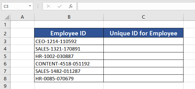
Lucky for us, the department name is followed by a hyphen '-', and the employee ID is 4 characters long. Now, we can use the MID function combined with the FIND function. The FIND function will locate the hyphen's '-' position, which will be the input value of start_num.
Use the FIND function as follows:
=FIND("-",B3)This formula locates the hyphen in B3 and returns 4 (the hyphen is the 4th character in B3). To use the FIND function as an input value for the start_num parameter, we must add 1 to this result because the unique ID begins from the 5th character of the text string and we don't want to see the hyphen in the final result.
The value of num_chars shall be 4 as all the unique IDs in our example are 4-digit numbers. So, combining the FIND and MID functions, the final function is as follows:
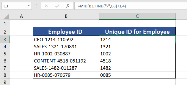
=MID(B3,FIND("-",B3)+1,4)And here's how this formula extracts the unique IDs for us:
Example 3: Extract First or Last Name
Imagine we have a data set of peoples' names and are asked to extract first, middle and last names in different columns. Usually, we would want to use the LEFT function for the first name and the RIGHT function for the last name. However, the functionality of two different functions can be accomplished using the MID function alone.
Let's learn how to extract first and last names using the MID function. We cannot simply use the MID function as the starting position for separating last names as the number of characters will vary for each name. Ergo, we will use the SEARCH function to our advantage and then merge it with the MID function.
We could have used the earlier mentioned FIND function too, but as we have understood the functionality of the FIND function, let's try to learn the MID function with the SEARCH function here. Also, the SEARCH function is case insensitive and that will make our task even easier.
Extract First Name using MID Function
The first and last names are divided by a space, a common pattern we can make use of. The beginning position in the MID function will be the starting of the string, whereas the number of characters can be determined using the SEARCH function.
The position of the space " " is where the first name ends and hence, is the number of characters to be extracted. The space character is located in the name using the SEARCH function, which returns its position, from which we deduct 1 to delete the inclusion of the extra space.
Let's try to put this logic in the form of an Excel formula.
Seeing the example ahead, the first name in cell B3 is 'Simon Rogers'. If we used the MID function only on this cell, we would try:
=MID(B3,1,5)However, this formula will not give us the required result for all other cells since all the names won't be 5 letters.
Let's generalize it so we can use it for the complete dataset.
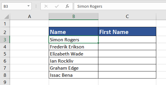
As the first parameter, start_num remains the same for all the names,. To determine the second parameter, we must find the position of the space. To find the position of the space " " using the SEARCH function, the formula will go as follows:
=SEARCH(" ",B3)Combining it with the MID function, the formula will become:
=MID(B3,1,SEARCH(" ",B3))To remove the extra trailing space, subtract 1 from the position. The final formula will be:
=MID(B3,1,SEARCH(" ",B3)-1)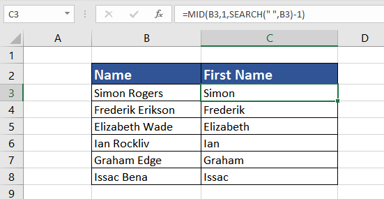
Furthermore, can we use the same logic to extract the last name? Let's find out.
Extract Last Name using MID Function
To pull out the last name using the MID function, we can use the SEARCH function to point out the start_num parameter as the last name begins after the space. How to find the number of characters (num_chars) to extract?
As mentioned earlier, if the total of the start_num and num_chars is more than the length of the string, the MID function returns the remaining string from the start_num. So, utilizing that to our advantage, there are two ways to use the MID function.
The first one is fairly simple. Assuming that the total character length of names will never exceed 1000, we can assign 1000 to the num_chars parameter.
The SEARCH function will determine the position of the space " " using the formula:
=SEARCH(" ",B3)This will be the input value of the first parameter start_num. Assigning 1000 to the second parameter, the formula will become:
=MID(B3,SEARCH(" ",B3),1000)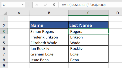
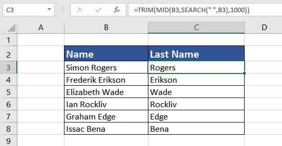
To remove the extra leading spaces from the extracted last names, use the TRIM function. The final MID function will be used as follows:
=TRIM(MID(B3,SEARCH(" ",B3),1000))Now we have the last names extracted by the MID and SEARCH functions and leading spaces removed by the TRIM function:
The second way is more elegant. Instead of an assumed number in the num_chars parameter, we can use the LEN function to determine the total length of the name and use that value in the num_chars parameter.
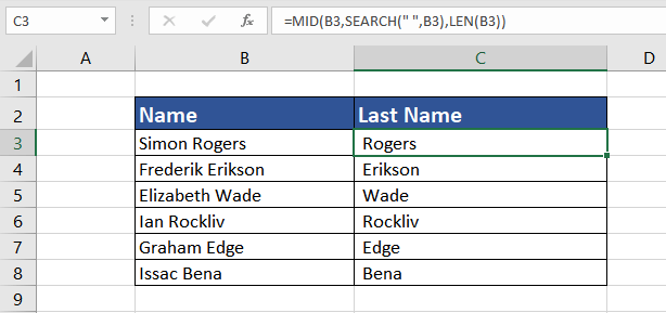
Combining the LEN & SEARCH functions with the MID function, the formula will be as follows:
=MID(B3,SEARCH(" ",B3),LEN(B3))Here, LEN function will return the total length of the input string, and SEARCH function will extract the position of the space " " in the string. The ultimate effect is similar to what we have seen in the previous formula. The location of the space character added to the total characters of B3 will obviously be more than the total characters in B3.
To polish it further, we can use the TRIM function to eliminate all the extra spaces.
=TRIM(MID(B3,SEARCH(" ",B3),LEN(B3)))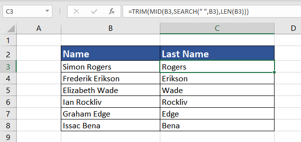
Substring Between Two Delimiters
After practicing the above examples, we can extract a substring from a string after determining the position of the space " " or any other special character. Now, what if the input string is long with several delimiters? Just for clarity, one or more characters that divide text strings are known as delimiters, such as space ( ), quotes ("), commas (,), semicolons (;), slashes (/) or pipes (|).
When we dive in further, there are two scenarios of extracting a substring from an input string between delimiters; first when they are different and second when the delimiters are the same. Let's understand both cases using an example.
Example 1 – Extracting Substring Between Two Different Delimiters
Let's assume we have a set of email IDs, and for research purposes, we want to extract the domain name from each email ID to analyze which one is most preferred. The email ID structure goes as follows '[email protected]', where 'learning' is a username and gmail is a domain name.
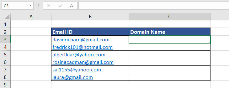
As we can see, we have two different delimiters (@) and (.) separating the domain name (gmail) from the rest of the string (username). So, to pull out the substring, we must locate the position of two delimiters where the first delimiter is the starting position (start_num), and using the second delimiter, we can calculate the number of characters to be extracted.
As we already know, the MID function consists of three arguments. The first argument is the cell reference to email ID (B3). The second argument is the starting position which can be calculated using the SEARCH function:
=SEARCH("@",B3)This formula will give us the position of the first delimiter (@). As we require the starting position to be one character after (@), we add 1.
Lastly, for the third argument (num_chars), we need the number of characters to be extracted. We can find the location of the second delimiter (.) and then subtract the position of the first delimiter. The formula goes as follows:
=SEARCH(".",B3)-SEARCH("@",B3)To finalize and remove the trailing space, subtract 1.
Putting it all together, the final MID function formula to extract the substring from two different characters is:
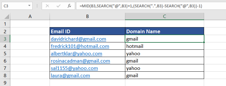
=MID(B3,SEARCH("@",B3)+1,(SEARCH(".",B3)-SEARCH("@",B3))-1)This is how our experiment turned out:
Example 2: Extracting Substring Between Same Delimiters
In the above examples, we already know how to extract the first and last name from the full name using the MID function. However, what about the middle name? We cannot simply use the basic MID function as the character length of middle names varies for each person.
However, in the previous example, we learned how to extract a substring between two delimiters.
As we will notice, there is a space ( ) before and after the middle name, separating it from the first & last name. We can find the position of two delimiters (in this case, both the delimiters are space characters) and extract the middle name from the full name.
In the given dataset in column B, we have the list of full names. Let's take the example of the first name in cell B3.

The first parameter of the MID function is the input text which is cell B3. For the second parameter, that is start_num, if we find the position of the space before the middle name and then add 1 to it, we should have our argument input. Using the SEARCH function, the position of the first space " " can be determined using the following formula:
=SEARCH(" ",B3)+1This returns 7 and if we do a quick count check, indeed the middle name's first letter is the 7th character of the text string.
Easy enough, right?
Now, to determine the number of characters to be returned, we can find the position of the second space " " (after the middle name) and subtract the position of the first space from it.
Remember, the SEARCH function has an additional third optional parameter start_num stating the starting position of the search within the string. This will come in handy here as there are two spaces in this text (full name). To find the position of the second space, the formula goes as follows:
=SEARCH(" ",B3,(SEARCH(" ",B3)+1)Explaining further, we are telling the SEARCH function to find " " in B3 starting after the position of the first space. If we don't use the nested SEARCH function, it will keep returning the position of the first space, and we don't want that, do we?
This formula returns 11 which you can tally again. Now that we have the position of both the space characters 11-7 is the number of characters to extract. Combining all to finish our MID function, the formula goes as follows:
=MID(B3,SEARCH(" ",B3)+1,SEARCH(" ",B3,(SEARCH(" ",B3)+1))-(SEARCH(" ",B3)+1))The MID function will return 4 characters from B3 starting from the character after the first space. The result is Dona and the rest can be seen below:

Forcing MID Function to Return Numbers
Like other text functions in Excel, the output value of the MID function is always in text format. Even if the input or output value contains only digits and looks like a number format, it is indeed in text format.
There are two ways to find if the output value is in text or number format. One is the innate nature of Excel to left align a text and right align a number. The second is to use the ISNUMBER function.
In this example, we multiply 99 with 200 and then extract the 2 digit of the result, starting from the second position. Using the MID function, the formula goes as follows
=MID(99*200,2,2)
We know that 99*200 is 19800. We are trying to extract 2 digits out of it starting from the 2nd position and hence the result is 98.
However, if you notice the result here is left aligned. By default Excel aligns all the numbers to right and text to left. This hints that the result here is a text instead of a number.
This can be further proved with the ISNUMBER function, which also returns false implying that the result of the MID function is not a number.
To ensure that the MID function returns a number, use the VALUE function, which transforms a text value representing a number into a number. Wrap the MID function inside the VALUE function. The formula used will be:
=VALUE(MID(99*200,2,2))
As evident from the example, the return value of the MID function combined with the VALUE function is right aligned, and when checked with ISNUMBER function, the result is TRUE.
RIGHT Function vs LEFT Function vs MID Function
We have now understood several ways to use the MID function for various tasks. Similar to the MID function, there are two more text functions in Excel; LEFT & RIGHT functions. For better comprehension, we will attempt to use all three Excel functions on the same input string in the following example.
In this example, we have taken an input text/string in cell A2 "Smart, Easy & Effective"

We have used the LEFT function to extract the first word of the string "Smart". As it is 5 characters long, the LEFT function formula will be:
=LEFT(A2,5)Unlike the MID function, the LEFT function doesn't have the start_num argument since the starting point is automatically the first character from the left. The same is the case with the RIGHT function. It just extracts characters from right to left.
Similarly, we've used the RIGHT function on the input string to extract the last word "Effective" (9 characters long). The formula is:
=RIGHT(A2,9)Now the function that we know very well; the MID function. The formula used to extract the middle word "Easy" will be:
=MID(A2,8,4)With that, we've discussed the ins and outs of the MID function. There are numerous other interesting things the MID function can manage such as returning a word beginning with a certain character (e.g. social media tags with the @ symbol such as @cholecakes, @popartillustrations), returning the nth word from a text string, and so on. Keep practicing and explore new ways to use the MID function.


