Excel MONTH Function – How To Use

The MONTH function is categorized as a Date/Time function in Excel and extracts the month component of a valid Excel date for us. The function returns an integer between 1 to 12. This return may be relayed to another function by nesting the MONTH function.

Syntax

The syntax of the MONTH function is as follows:

Arguments:

'serial_number' – This is a required argument where you will need to add the serial number for the date or a cell reference to a cell containing such date, from which you want to extract the month component.

Important Characteristics of the MONTH function

• The MONTH function always returns an integer from 1 (January) to 12 (December).
• The cell displaying the return may be formatted to display the name of the month instead of a number between 1 and 12.
• The date in the serial_number argument may be supplied as a serial number, a valid text date (for instance: "25-Dec-2001"), as a nested DATE function, or as a nested TODAY function.

Examples

Let's try to see some examples of the MONTH function.

Example 1 – Plain Vanilla Formula for the MONTH Function

We'll start by looking at the lay of the land with a basic MONTH function formula. Let's take a date and extract its month component using the MONTH function, like so:

As shown in the example, we receive the same output with the following formulas as well:

With the date 25 December 2001 supplied as the serial_number argument, the formula returns 12. It's a simple function that perpetually returns an integer value — so, let's add some colors to this function and make the output look more vibrant.

Example 2 – Highlight Dates of the Current Month

We have a rather long list of dates, all jumbled up. Those are the dates for our bank transactions, and we want to reconcile transactions for a certain month. Instead of skimming through the entire list, we can have Excel highlight dates from that specific month.

To do this, we'll use the following formula for conditionally formatting the cells:

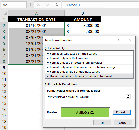
Select the range of cells containing the list of dates and create a New Rule from the Styles section under the Home tab. Format the cells with a green fill or another color of your liking. This should give you the output as shown in the above image.

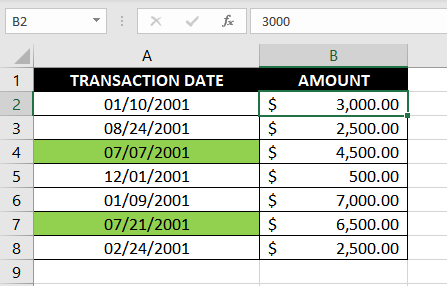
What we're doing here is checking if the returns from both the MONTH functions are equal. If you wish to do the reconciliation for a different month than the current one, all you need to do is instead of using the TODAY function, pass any arbitrary date of that month.

The formula returns a Boolean value. If both MONTH functions return the same integer, the formula returns TRUE and FALSE otherwise. If the returned value is TRUE, the cell gets highlighted.

Example 3 – Check if a Certain Year is a Leap Year

We're now clear with the basics; let's move on to some more logical formulas now. We're going to try and verify if a certain year is a leap year. To do this, we'll use a combination of the MONTH, DATE, and YEAR functions.

Here's the formula we'll use:

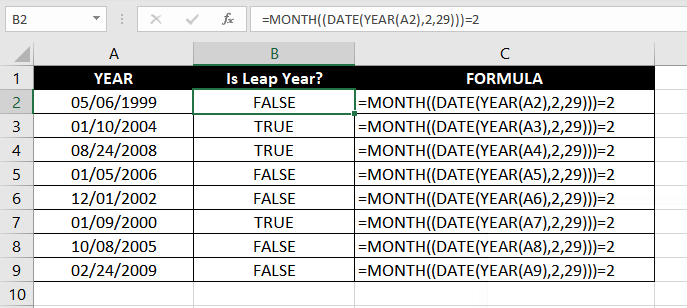
The formula may look bulked up because there are three functions in there. In reality, though, the formula's logic isn't that complex.

The YEAR function is the entry point from where our input enters the formula. For instance, our first row has the year 1999. This value is relayed to the DATE function. Therefore, the DATE function's output will be February 29, 1999.

However, the date February 29, 1999, is invalid. Therefore, the DATE function's output will default to the first day of the next month, i.e., March 1, 1999.

By now, you probably know how the formula works. If a certain year has an extra day (i.e., February 29), the MONTH function will return 2 (for February), and 3 (for March) otherwise. If the MONTH function returns 2, the condition holds and the formula returns TRUE. If the MONTH function returns 3, the formula returns FALSE.

Example 4 – Get Month Number from Name using MONTH function

What we want to do now is convert a list of month names to a number (i.e., 1 for January, 2 for February…). To accomplish this, we'll use the MONTH function in combination with the DATEVALUE function, like so:

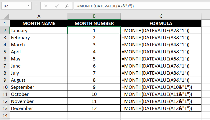
If you know what the ampersand (concatenation operator) does in a formula, you'll know right away what this formula is trying to do. For the uninitiated, we'll break the formula down.

The DATEVALUE function converts a text string to a valid date. In our case, the function picks up the text string (i.e., January, February…) and attaches 1 to it (that's what the ampersand does). So, the text string supplied to the DATEVALUE function is January 1, February 1, and so on.

Notice that we still haven't added a year component. That's because we don't need to. The DATEVALUE function returns the current year by default. Therefore, in our case, the DATEVALUE function returns January 1, 2021, to the MONTH function.

MONTH function's purpose remains the same here. It now has a date as its argument, and it just needs to extract the month and return the appropriate integer value.

Example 5 – Get Fiscal Quarter from a Date

Let's say we have a list of dates and we want all dates that occur in quarter 3 of a certain fiscal year. While there is no specific formula to do this, it just requires some knowledge of an Excel  CHOOSE function and some elementary logic.

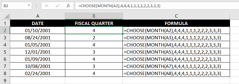
The first argument in the CHOOSE function is an index number that works as a reference for the values entered in the following arguments. For instance, if the first argument is 4, the CHOOSE function will return 1.

The return of the MONTH function works as an index number in this formula. If the date in cell A2 occurs in January, the MONTH function will return 1. Consequently, the CHOOSE function will return 4.

In this example, we've assumed the first quarter as April to June and the last quarter as January to March. Therefore, the first three values in the CHOOSE function following the index number are 4 — they represent the first three months of a calendar year (January – March). If you want to assume the first quarter as October to December, the first three values would all be 2s since in that case, the months January to March would occur in the 2^nd quarter.

With that, we've discussed the ins and outs of the MONTH function. It's a simple, but extremely handy function when you want to play around with dates in your worksheet. Practice these formulas and before long, they'll become second nature. By the time you're through, we'll be waiting for you with another Excel function.