Excel REPT Function – How To Use

The REPT function in Excel is used to repeat the input text a given number of times. Irrespective of the format of the input text to be repeated, the return value of the REPT function is always a text value.

The REPT function is beneficial in creating histograms or in-cell charts for analysis or financial modelling.

Syntax

The syntax of the REPT function is as follows.

Arguments:

The REPT function accepts two mandatory arguments, and the details of each parameter are mentioned below:

'text' – This argument is the input value that we want to repeat using the REPT function. The text argument can be in any format, such as alphabet, string, numbers, or special characters.
'number_times' – This argument suggests the number of times that the input text is to be repeated.

Important Characteristics of the REPT Function

Some notable features of the said Excel function are as follows.

• If the value of the number_times argument is 0, the REPT function returns an empty cell.
• If a negative value is used as an input for the number_times argument, the REPT function results in a #VALUE! error.
• If a decimal is used as an input value for the number_times argument, the REPT function ignores the decimal and only considers the integer value.
• The REPT function returns a #VALUE! error if the result of the REPT function is longer than 32,767 characters.

Examples of REPT Function

As we have already understood the basic syntax and the characteristics of the REPT function, let's explore additional applications and ways to utilize the REPT function to our advantage.

Example 1 – Simple Use of REPT Function

In this example, we will learn the basic functionality of the REPT function with different input values for both arguments. We have covered all possible combinations for a better understanding.

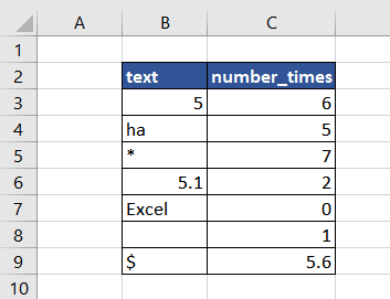
The formula used will be as follows.

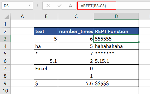
As observed, the REPT function behaves similarly for numbers, text, characters, decimals, and strings. It simply repeats the input value of the text argument the number of times specified by the second argument, number_times.

In the first example, the REPT function repeats '5' six times, returning the value '555555'. The same is the case for the following four examples.

In cell D7, the REPT function is asked to repeat 'Excel' zero (0) number of times; hence, the final return value is an empty cell. The same is the case in cell D8; when an empty cell is asked to be repeated once, the return value is an empty cell.

In the last example, we can observe the above-stated characteristics that the REPT function truncates the decimal value when it is used as input for the second argument. The REPT function only considered the integer value 5 and hence repeated the '$' five times, returning the value '$$$$$'.

Example 2 – Creating In-cell Chart Using REPT Function

One of the most known and functional applications of the REPT function is creating different charts, such as in-cell charts and dot charts, for more visual data representation. Here we have the monthly sales for the entire year.

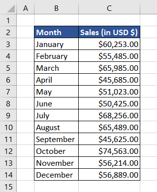
Analyzing them will become easier if the sales are illustrated in a chart format. Using the REPT function, we can easily illustrate the sales data in charts. The Unichar code for a block is 9612 and we will user UNICHAR function to display it.

The formula will be as follows.

Here in this formula, we are trying to repeat UNICHAR(9612) for C3/10000 times. We chose to divide the value in column C by 10000 since we are displaying the sales in the multiples of 10000 and for ease of presentation.

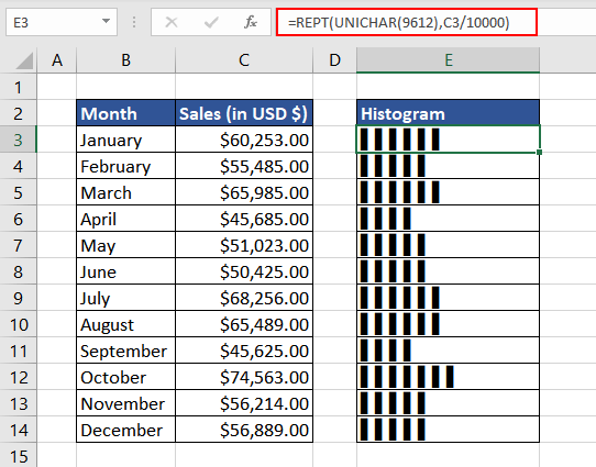
Now we can analyze the data in a matter of minutes. To add on, we can simply suffix the total sales in each in-cell histogram to make a complete representation of the yearly sales. The formula used will be as follows.

Along with the REPT function used above, we have added the DOLLAR function and the text representing sales in that month. We have used the DOLLAR function instead of directly using the cell reference to avoid losing the currency formatting.

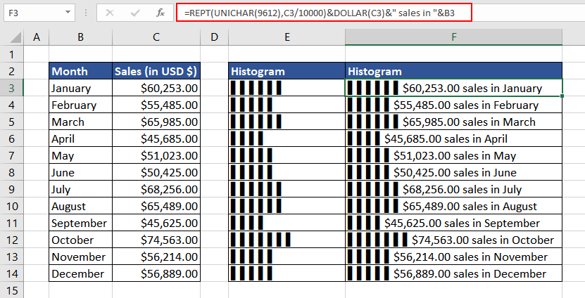
Hereon, column F can be used directly as our yearly sales report.

Now that we have understood how to create in-cell graphs, let's take a step further and curate a tally chart using the REPT function.

Example 3- Creating Tally Charts using the REPT Function

In this example, we are creating a tally chart for the count down to the number of days left for the next holiday. The REPT function is an excellent way to achieve that. So here we have a list of all the upcoming holidays, and when we enter today's date in cell C2, it will create a tally chart for the number of days left.

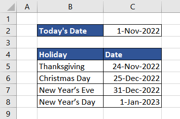
We will simply use the following formula to calculate the number of days left. Subtract today's date from the holiday date. We are also fixing the cell reference of today's date by using the $ sign. For better understanding, you can also read what does dollar sign ($) mean in Excel formulas?

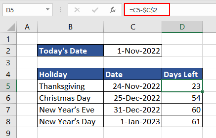
We will use a combination of two REPT functions. The first REPT function represents tally marks, and the next shows the remaining count.

As the REPT function only considers the integer value in case decimal numbers are used as an input value for the number_times argument, we will divide the number of days by 5 to create a grouping for the tally chart. The formula used will be as follows.

As we can see here in the first case, the number of days is 23 and, using the first part of the REPT function, the tally chart shows 20. To display the remaining days, we will use the MOD function to extract the remainder after the number of days is divided by 5. The formula used will be as follows.

Finally, combine both the REPT functions to display the countdown tally chart. The final formula used will be as follows.

Now with today's date entered, you can see the tally chart become smaller as the holidays approach.

Example 4 – Pad Text for Equal Length

Here in this example, we have a first and last names dataset. To ease the data entry process, we must ensure that all the first names are of the same length, followed by the last names of equal length. To do that, we can add or pad the first and last name with additional spaces or characters. Let's see how to do that using the REPT function.

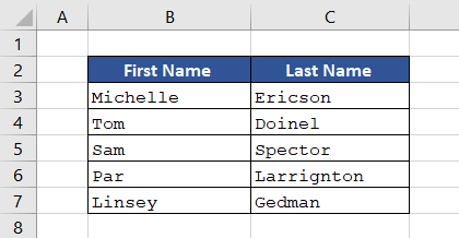
Assuming that we need the first and last name to be 10 characters long, we will use the REPT function to add a variable number of spaces and asterisks (*) to each name until all of them are of equal length.

We will use the LEN function to calculate the number of spaces and asterisks to be added to the first name and last name. Subtract the length of the name from the total, which is assumed to be 10 in this case. The formula used will be as follows.

So, putting it all together, starting with adding the first name with the number of spaces to ensure the length is 10, then adding the last name with the number of asterisks to make up to 10-character length. The final formula used will be as follows.

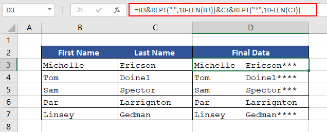
The data in column D is formatted with a monospaced font (Courier New) to show that all strings are the same length.

Example 5 – Finding the Last Text in Column

We have downloaded a list of top movie names from the internet. Now, we want to begin watching the movies in ascending order of popularity, saving the best one for the last. So, we will try to extract the last movie name from the list. But as it is downloaded, it also contains some random numeric data, which might interfere with our task.

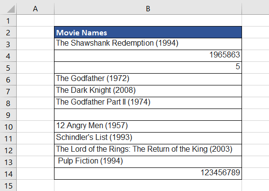
Using the REPT and VLOOKUP functions, we will extract the last text from column B.

Excel works like a dictionary where 'z' is the largest and 'a' is the smallest letter. So, the letter 'z' repeated 100 times can be assumed to be the biggest word. Now, combining that logic with the basic functionality of the VLOOKUP function looking for an approximate text match can help us.

When using the approximate match in the VLOOKUP function for text, it assumes that the data is in ascending order and, therefore, the closest match to the largest text would be the last text in the column. It considers the last text value as the largest and closest value to z being repeated 100 times.

The formula used will be as follows.

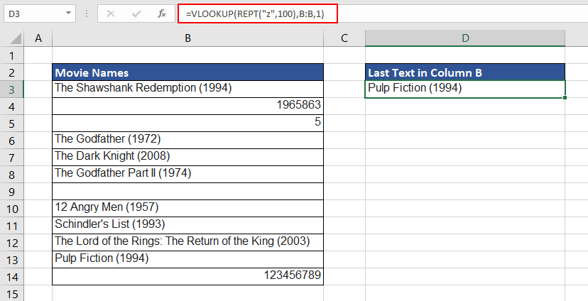
As we can see, the Excel function omitted the last value of column B as it was a numeric value and returned the last movie name, which was also the last text value.

Hopefully, you have comprehensively understood the different features and applications of the REPT function. Try them on your own and discover new ways to fully utilize this exciting Excel function until we come back with the next one.