Excel ROW Function – How To Use

The ROW function retrieves the row numbers of a given cell, range of cells, or array. It is a versatile function and is useful in Conditional Formatting and when dealing with large datasets. The ROW function can also be combined with other Excel functions to create solutions as per our needs.

It is worth noting that the ROW function returns the row number relative to the number of the topmost row in the worksheet. The first row in the worksheet will be 1, the second row will be 2, and so on.

Syntax

The syntax of the ROW function is as follows.

Arguments:

The ROW function accepts one argument which is optional.

'reference'- It includes the cell or range of cells whose row number(s) we wish to extract. If the reference argument is left empty, the ROW function shows the cell's row number containing the formula.

Important Characteristics of the ROW Function

Some noteworthy features of the ROW function are as follows.

• The input value of the reference argument can be a single cell address or a range of cells. As it is an optional argument, it can also be left empty.
• The reference argument cannot include multiple references or addresses.
• If the at symbol (@) is added as a prefix to the ROW function, Excel doesn't interpret the input value as an array but considers it as a single value. The at symbol (@) is also called an implicit intersection operator.

Examples of ROW Function

Although the ROW function may appear simple at first glance, there are several applications that can aid your productivity. Let's deep dive into various examples and explore different applications of the said function.

Example 1 – Simple Use of ROW Function

In this instance, we have taken different input values of the argument reference to understand the function in a comprehensive manner.

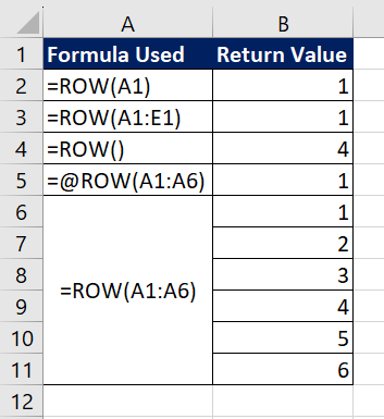
The first case is straightforward where the input value of the argument is a single cell reference i.e. A1. The ROW function returns the row number which includes the cell reference A1 and thus the return value is 1.

In the next instance, the input reference value is a cell range A1:E1. As all the cells in the range are in row 1, the ROW function returns 1. As stated already, when the argument is left empty, the ROW function returns the row number of the cell containing the formula. In the third case, the formula is placed in cell B4, therefore the return value is 4.

The next example showcases one of the exclusive attributes of the ROW function. When the at symbol (@) is added at the beginning of the function, it is an indication to Excel to disable array behavior and treat the input array as a single value. Even if the input value in this example is A1:A6, the return value is 1 as the ROW function only returns the row number of the first value which is A1.

The last example shows how the ROW function behaves with a range of cells or arrays. The input value is A1:A6, to which the function results in row numbers of each cell in the range which is {1,2,3,4,5,6}.

Now that the basic functionality of the ROW function is clear, let's explore other examples.

Example 2 – Creating Sequence with ROW Function

As the ROW function returns the row number of the cell containing the formula, it is an excellent tool to create sequential numbers. In this example, we have employees' names and their department names. We now wish to create employee IDs for all.

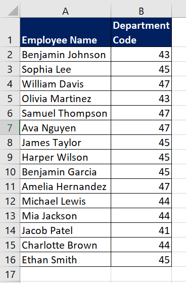
Using the ROW function, we can create sequential numbers or IDs which can be concatenated with department code. We will use the ROW function without a cell reference hence it will return the row number of the cell where the formula is entered.

The formula used will be as follows.

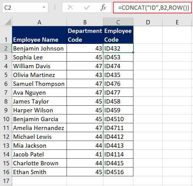
After we dragged the formula to cover the complete dataset, we now have unique IDs for all the employees.

Example 3 – Adding Value on Every 3rd Position

In this example, we have a list of products that are sold at a furnishing store. The existing process followed is to use product names as product codes. We now wish to change the convention and use unique product codes. To test it out, we would assign a unique code to every 3rd product.

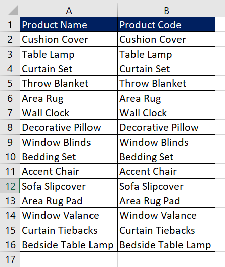
The naming convention that we wish to follow for every 3rd product is "PRD-000X", where X represents a unique digit which can be the corresponding row number. All the other products will contain the product names copied from column A.

To find every 3rd row, we will combine the ROW and MOD functions. The ROW function will return the current row number while the MOD function will calculate the remainder when the row number is divided by 3. For every 3rd row, the MOD function shall return 0.

The formula used to find the current row number is as follows.

1 is subtracted from the ROW function to adjust the row number by one as the first row contains headers.

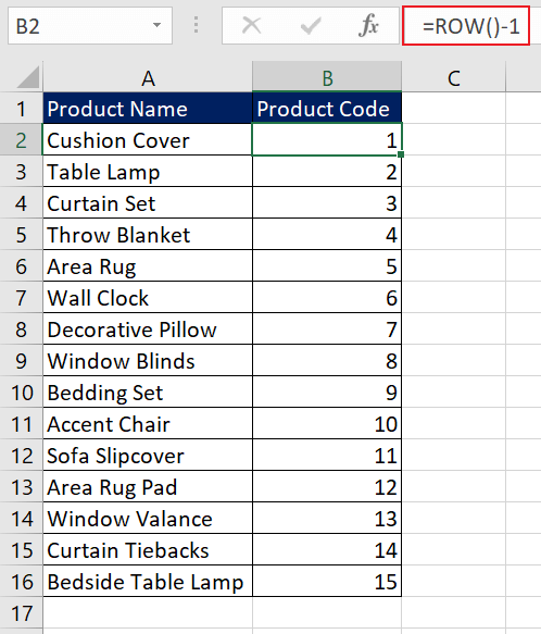
Now, wrapping it in the MOD function, the formula will be as follows.

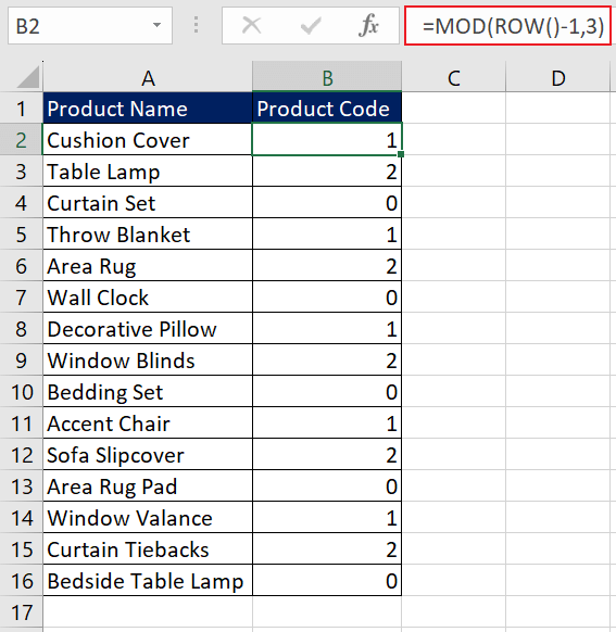
Finally, use the IF function to add the "PRD-" prefix with the row number formatted as a 4-digit number – if the return value of the MOD function is 0.

The formula for the logic will be as follows.

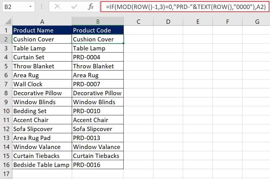
Using the same logic, we can perform specific operations on every nth position in a column. Try using it to perform calculations on specific rows or positions in your data based on predefined rules or requirements.

Another excellent use of the ROW function is in combination with the INDEX function to create dynamic results. Let's delve into an example to illustrate this further.

Example 4 – Creating Smaller Dataset with ROW Function

Suppose we downloaded the stock prices of a company we wish to invest in from the internet. As it is a large dataset, we wish to create a smaller dataset based on specific dates for easy analysis.

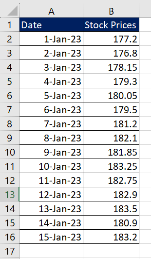
To improve the experience further, we can select two cells where the user can enter starting and ending dates. In this case, they are E2 and E3. To create a smaller dataset, we will use two steps which include the INDEX and ROW functions.

The INDEX function will be used to retrieve the corresponding stock prices from column B based on the row numbers. To get the desired row numbers, we will use a combination of ROW and INDIRECT functions.

Using the cells E2 and E3, where the users enter the row numbers, the formula used will be as follows.

We are adding 1 to the starting day and last day as the first row contains column labels. Then, combining both the input dates to create a cell range as text strings separated by a colon. The INDIRECT function will then return a cell reference specified by the text string. Finally, we wrap the INDIRECT function in the ROW function to get a list of row numbers within the specified range.

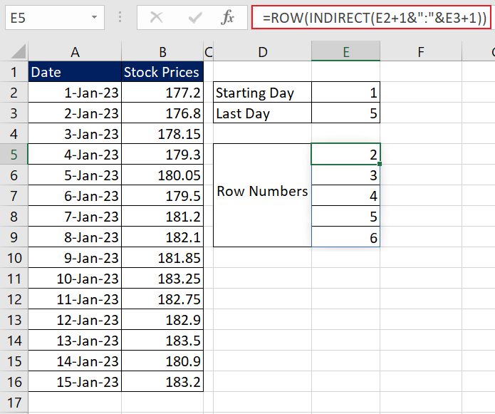
The next step is to use the INDEX function to extract the data from column B based on the row numbers. The formula will look like this.

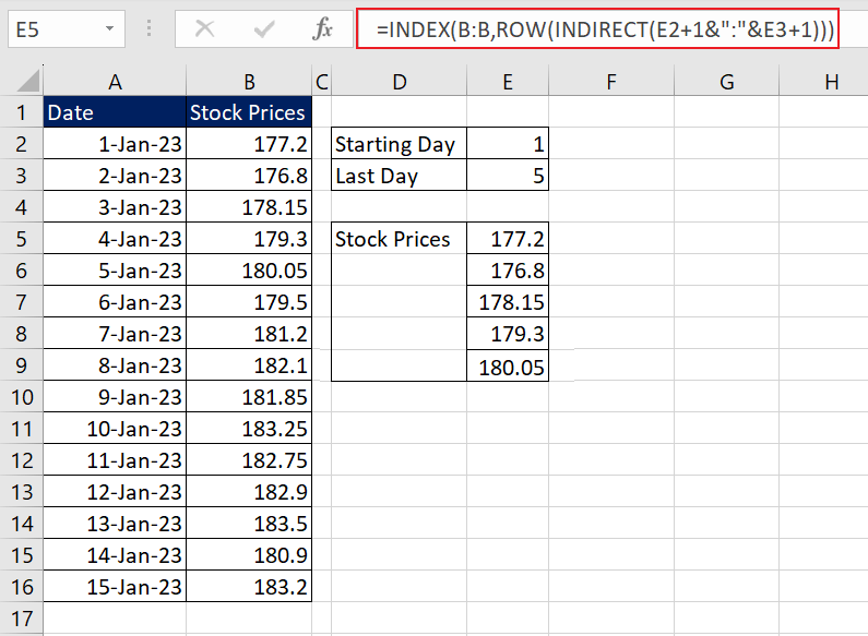
For further analysis, spending on the requirement, we can also calculate the average prices of given days by wrapping the above-mentioned function in the AVERAGE function. The updated formula will be as follows.

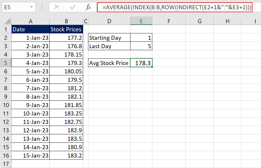
ROW Function vs ROWS Function

Both the ROW and ROWS functions in Excel are useful when dealing with large datasets.

Now, we know that the ROW function returns the row number of a given cell or range of cells. On the other hand, the ROWS function is used to count the number of rows in a range of cells or arrays.

One noteworthy difference between the ROW and ROWS functions is that the argument in the ROW function is optional whereas it is mandatory in the ROWS function. Let's understand both functions with an example.

Here, we have a sample dataset where we used both functions in a simple manner. The formulas used are as follows.

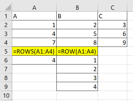
The ROWS function counts the total number of rows in the cell range A1:A4, which turns out to be 4. The ROW function gave the row numbers of each cell included in the cell range A1:A4.

By utilizing a combination of the ROW and ROWS functions, we can effectively determine the position of the last row within a specific cell range. It is crucial to clearly understand the distinction between these two functions, as their names can be easily confused.

ROW Function vs COLUMN Function

As the ROW function retrieves the row number of a given cell reference or array, the COLUMN function returns the column number of the specified cell or range of cells.  Let's take a simple dataset to understand the difference.

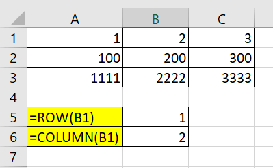
In the above dataset, both functions include the same input value. The ROW function returns the row number of cell B1 which is the 1st row, whereas the COLUMN function results in the column number of cell B1 which is the 2nd column.

Although the ROW function appears basic, practice to discover more applications to improve your data analytics skills and productivity in general. While you master this, we will bring you another useful Excel function to add to your arsenal, which will further enhance your ability to navigate through large datasets.