Excel TEXTAFTER Function – How To Use

The TEXTAFTER function returns the text that appears after a given character, substring, or delimiter. If the delimiter is used more than once, we can also choose to extract the text after a particular occurrence of the delimiter.

The TEXTAFTER function is one of the latest additions and currently only works with Microsoft Excel 365.

Syntax

The syntax of the TEXTAFTER function goes as follows:

Arguments:

The TEXTAFTER function contains six arguments, out of which two are mandatory. The details of each argument are mentioned below.

'text' – This is a mandatory argument that accepts the input text from which we wish to extract the subtext. It can be a direct value in double quotes or a cell reference.

'delimiter' – This is also a mandatory argument. The value of the delimiter is a character or substring that points to a place after which we wish to extract the text.

'instance_num' – This is an optional argument that indicates the nth occurrence of the given delimiter, after which we intend to extract the text. The default value of instance_num is 1. If the value of instance_num is negative, the function looks for the delimiter from right to left.

'match_mode' – This is an optional boolean argument that only accepts 1 or 0 as its input value. The default value is set to 0, which makes the TEXTAFTER function case-sensitive. On the contrary, the function is case insensitive when the value is set to 1. The value of the match_mode argument indicates the function of whether to perform a case-sensitive match with the delimiter or not.

'match_end' – It is an optional argument that accepts a boolean value of 1 or 0 as input. The value of the match_end determines if the end of the input text will be considered as the given delimiter. The default value of match_end is set to 0, meaning the end of the text will not be considered the delimiter, and when set to 1, the end of the text is assumed to match the given delimiter.

'if_not_found' – This is the last optional argument and contains the value we wish to return if the given delimiter is not found in the given text. By default, #N/A is returned.

Important Characteristics of the TEXTAFTER Function

One of the most basic features of the TEXTAFTER function is its categorization as a text function; the return value is always in text format. Other important attributes of the TEXTAFTER function are as follows:

• If the text argument is empty, the function throws a #VALUE! or #N/A error.
• The value of the instance_num argument is an integer value. If the input value is decimal, only the integer part of the value is considered.
• If the value of the instance_num argument is 0 or is more than the length of the input text, the TEXTAFTER function results in a #VALUE! error. If the value exceeds the number of delimiter occurrences, a #N/A error will show.

Examples of TEXTAFTER Function

As there are many arguments in the TEXTAFTER function, go through the below-mentioned examples to better understand their usage.

Example 1 – Simple use of TEXTAFTER Function

Here, we have taken a basic data set to understand the vanilla functionality of the TEXTAFTER function.

In the first example, the input text is a simple string where we wish to extract text after the at sign (@), which will be used as the input value of the delimiter. The return value is as expected in cell C3.

In the second example, the value of the text argument is in numerical format. We intend to extract the characters after the number 5. The return value in cell C4 is after the first occurrence of the number 5. This is because the default value of the instance_num argument is 1; therefore, the first instance of the delimiter 5 is noticed, and the text after that is returned. Also, note that the return value in cell C4 is in text format, as is evident by its left alignment.

In the third and fourth examples, the delimiter is missing. As it is empty, the TEXTAFTER function matches the empty delimiter right at the beginning of the text and returns the complete text, as seen in cell C5. In the last example, the delimiter is empty, but the value of instance_num is negative. Therefore, it matches the empty delimiter right at the beginning, which is the end of the string in this case and returns an empty cell.

Hope you now understand the basic functionality of the TEXTAFTER function. Other uses and applications of the function are explained in detail below.

Example 2 – Extracting Names Using TEXTAFTER Function

Here, we have extracted all attendees' basic greetings and names. We now intend to extract the names from the string for data entry.

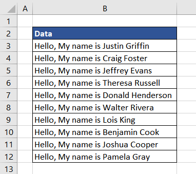
Using the TEXTAFTER function, we can easily pull out the names after the word 'is' as it is only used once in the text. Since there is a space after the word 'is', we will add it to the input value of the delimiter. The formula used will be as follows:

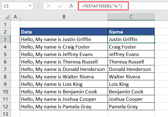
In this case, space can also be used as a delimiter. So, another way of separating the names from the string is to use space as a delimiter and use the argument instance_num as there is more than one space in the input string. The names in the input string are after the 4th space. Therefore, the formula used will be as follows:

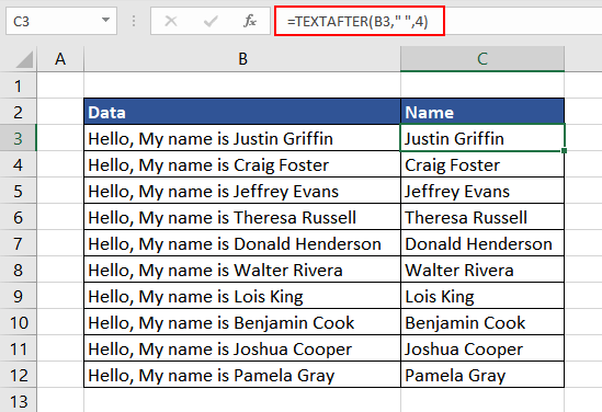
Example 2.1 – Understanding match_mode argument of TEXTAFTER Function

Continuing the previous example, this time, the data received has inconsistent case types. Again, we are trying to extract the names in a separate column. The formula used is the same as before.

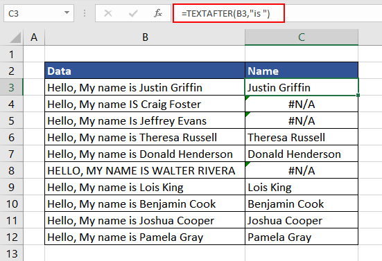
As the default nature of the TEXTAFTER function is to make a case-sensitive match with the delimiter, it cannot match the delimiter in the original text string, and therefore it returns a #N/A error. To ensure the match is case-insensitive, we set the value of the match_mode argument to 1 or TRUE. The formula used will be as follows:

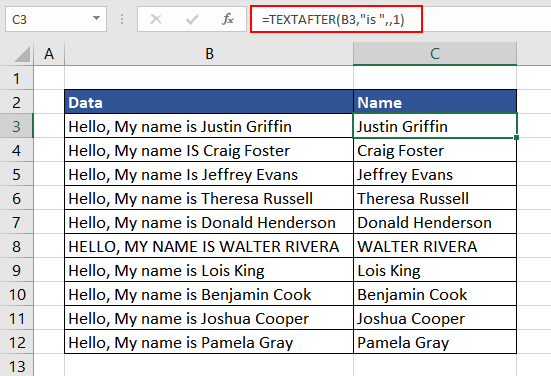
Now we have all the names separated. In this example, the delimiter used in the data was consistent. What happens if the separator or delimiter varies across the data?

Example 3 – Using Multiple Delimiters in TEXTAFTER Function

In this instance, we have a database containing people's names, ages, and occupations. From this database, we wish to extract occupation in a separate column.

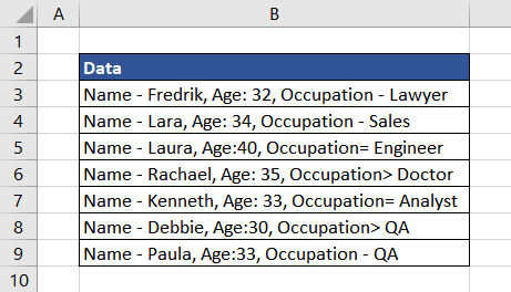
As we can see, the character used after the word "Occupation" varies across the data. Therefore, if we wish to extract the occupation from each string using the TEXTAFTER function, multiple delimiters will be used.

Here, we will use a dash(-), equals to sign (=), and greater than sign (>) as delimiters. To use multiple delimiters, in the TEXTAFTER function, they must be used as array constants in curly brackets, each delimiter enclosed in double quotes, separated by a comma. The formula used will be as follows:

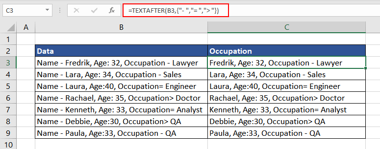
The result value in column C is different from what we expected. This is because the TEXTAFTER function encounters the first delimiter, which is a dash (-), at the beginning of the string and returns the rest of the string after the first dash. To prevent that, we must mention which occurrence of delimiter must be included. In this case, the last occurrence of the delimiter must be included for the required result.

If the value of the instance_num argument is negative, the function counts the occurrence of delimiters from the end of the string. We can use that to our advantage, and the formulated function will be as follows:

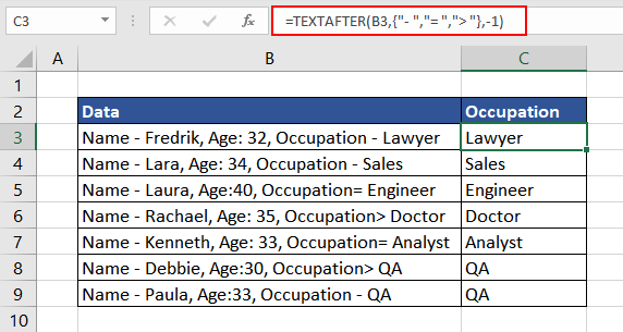
We finally have the desired data. The same data can also be retrieved using the combination of the RIGHT function with the SEARCH and LEN functions.

Example 4 – Calculating Sum Using TEXTAFTER Function

In this case, an online request was sent enquiring about the prices of a few mobile phones. We have received the prices for the same, but as they are combined with text, further calculations cannot be performed.

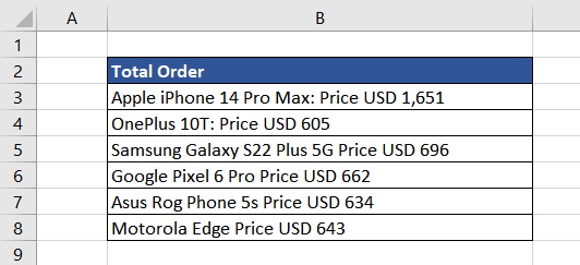
To get the total cost of the phones, we can use the TEXTAFTER function to extract the prices and then calculate the sum. Let's understand it one step at a time. To get the prices in a separate column, the following formula will be used where the delimiter is 'USD'.

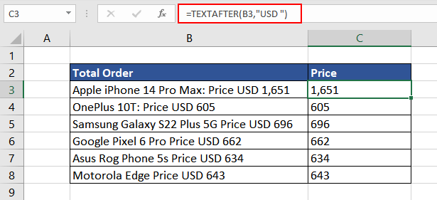
The data is in text format, as evident from the left alignment of the prices in column C. So, no mathematical calculations can be done. First, we must convert the return value into the numeric format and then wrap everything in the SUM function.

To ensure everything can be performed in one step, we will change the cell reference from only B3 to the complete range B3:B8. Converting the return value in numeric format, the formula used will be as follows:

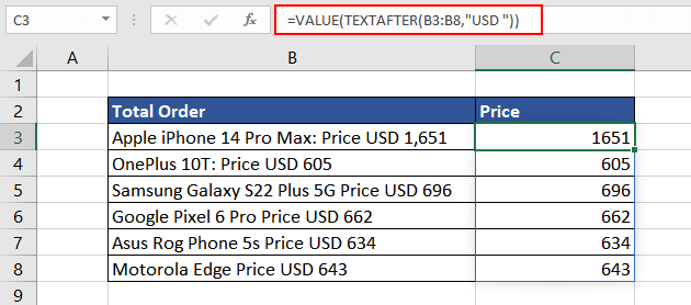
Now, finally, we can calculate the total sum of prices. The final formula to be used is as follows:

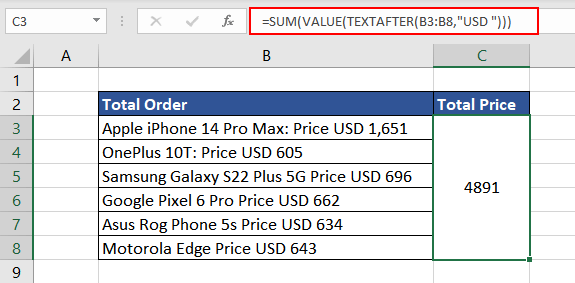
By now, we have understood the usage of the first four arguments. The next example is curated to provide a clear understanding of the last two arguments.

Example 5 – Extracting Email IDs Using TEXTAFTER Function

In this example, we have the names and email IDs for the upcoming newsletter. As the data was user generated, few email IDs contain extra non-essential characters.

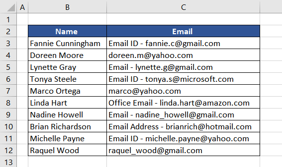
Looking at the data, we aim to extract the email IDs in a separate column. As we can see, the separator used is a dash. For entries where the delimiter is not present, we wish to return the email ID itself. The formula used will be as follows:

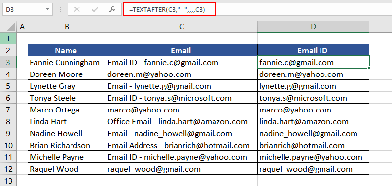
Finally, we have the email IDs in a separate column without any unnecessary characters. However, there is another way to get the desired result.

Instead of using the last argument, if_not_found, we can set the value of instance_num to -1. This way, the TEXTAFTER function starts looking for the delimiter from right to left. Now, in cases where the delimiter is not found, set the value of match_end to 1, which assumes that the given delimiter is present at the end of the string.

As we are looking for the delimiter starting from the end of the string, if it is not found, the function returns the complete input text as it is taken that the delimiter is present at the end of the string. In this case, it is the beginning of the string due to the negative value of instance_num. The formula used will be as follows:

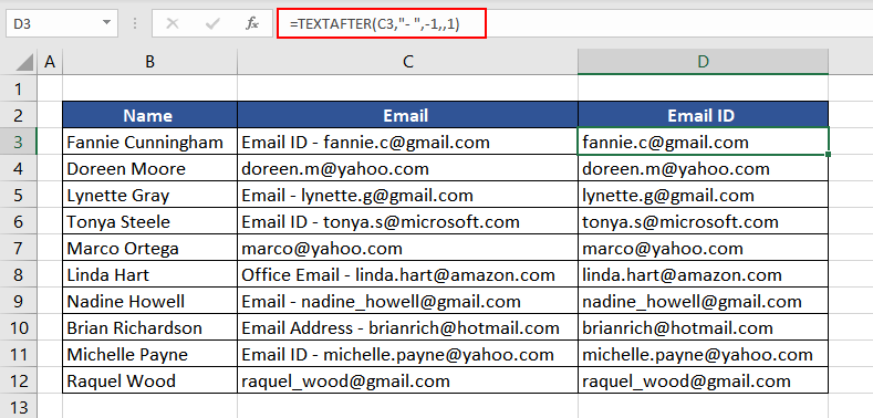
TEXTAFTER Function vs TEXTBEFORE Function

By now, we already know that the TEXTAFTER function extracts the part of the text after the given character or string. On the other hand, the TEXTBEFORE function returns the text that appears before the given character or string. Let's understand the difference better using the example given below.

Here, as the input text, we have the full name, which includes the first, middle, and last name separated using a space. We will use the TEXTBEFORE function to extract the first name before the first space and the TEXTAFTER function to get the last name after the last space. The combination of the two will return the middle name.

For the first name, the formula used is simple, where the delimiter is space.

For the last name, as we wish to extract the text after the last occurrence of space, we will use the value of instance_num as -1 so that the function starts the search from right to left. The formula used is as follows:

The return value is as expected in cell D4. Now for the middle name, first, we will use the TEXTAFTER function to extract the text after the first occurrence of space. The return value will be the middle name followed by the last name. Then we will use the TEXTBEFORE function on the return value, extracting the text before the space, giving us the middle name as seen in cell E4. The formula used will be as follows:

Hopefully, now, when you are dealing with a large dataset of text, the TEXTAFTER function will make tasks easier for you. Practice and discover new ways to use the given function while we curate an explanation of another interesting Excel function for you.