Excel UNICHAR Function – How To Use

The UNICHAR function in Excel returns the Unicode character or symbol associated with the given number. Unicode is a global encoding standard in which each letter, number, or symbol is assigned a distinct numeric value applicable across many platforms and programs.

The numbers, alphabets, characters, and symbols we see on the computer are actually stored as Unicode, where a unique number is assigned to each. The UNICHAR function returns the character corresponding to the supplied input number.

Syntax

The syntax of the UNICHAR function is as follows:

Arguments:

'number' – is a mandatory parameter. It is an integer value corresponding to a character or a symbol in Unicode. The input argument can be a number entered into the function directly or passed as a cell reference.

Important Characteristics of the UNICHAR function

The UNICHAR function is an upgraded version of the CHAR function and is categorized as a text/string function in Excel.

• When the input argument is invalid, the UNICHAR function will return a #N/A error.
• If the input argument number is zero or the number is outside the acceptable range, a #VALUE error occurs.
• For input numbers 1 through 255, the UNICHAR function returns the same characters as the CHAR function.

Uses of UNICHAR Function

Before jumping to the examples let's take a helicopter view and try to understand why do we need UNICHAR function in first place.

The original coding system was different as we followed the ANSI code system for Microsoft and the Macintosh character set for Apple/Mac OS. When users attempted to translate character codes from one system to another, they ran into issues. A universal character set, the Unicode system, was created to solve the problem. The first 255 code points of the ANSI and Unicode systems are identical for convenience.

There are several uses of the UNICHAR function in Excel. In Excel, special character symbols from the Unicode character set like ☐, ☑, ⚐, ⚑, ▲ can be used for various purposes. They can be used in charts, marketing copy, and in-cell pictograms. We live in the social media era and, therefore, cannot run away from the use of emojis. UNICHAR function helps us to add of these to our boring spreadsheets.

If we divide the Unicode into sections, different symbols have different applications.

0-32 are control characters like newline, tab, etc., 65-90 return uppercase English alphabets, whereas 97-122 return lowercase English alphabets.

If we are writing Swedish names such as Pär, Käthe, Påvel or Chlöe and we don't have a Swedish keyboard, the characters returned by the UNICHAR function using the codes from 196 to 214 come in handy.

So, when we wish to add other language alphabets different from the normal English alphabets, the function is useful although up to this point and until 255, the CHAR function can also be used.

UNICHAR function is also helpful when we want to add superscripts and subscripts (Unicode 8304 – 8351). Currency symbols, Greek characters, number forms, Roman numerals, mathematical operators, arrows, geometric shapes, braille patterns, musical symbols, etc. can all be added using the UNICHAR function. It also allows us to add playing card symbols, domino tiles symbols, and all kinds of emoticons.

Examples of UNICHAR Function

There are several ways to include special character symbols in Excel. We can use the Symbol option in Excel (Insert > Symbol). Both the symbol's name and the character code are provided, but the options are fewer. Another alternative is to simply copy and paste from the web.

But if we wish to include them in other Excel formulas, we can use the UNICHAR function.

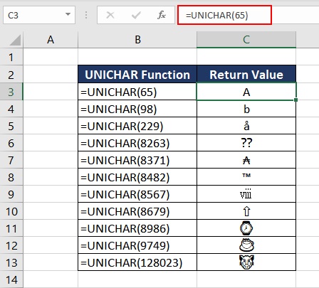
Here, we have taken numerous examples of directly using the UNICHAR function. You can notice that different Unicode (number argument) returns different characters or symbols.

Example 1 – Adding Tear Here Sign

We have often seen a 'Tear Here' dotted line at the end of official forms, acknowledgments, or invoices where one party can tear off a section of the document for their use. Have you ever wondered how to add those when creating such a document in Excel?

Using the UNICHAR function, we can easily add the tear here line to any document. So, in this instance, suppose we have to add one in the invoice, where the 'tear here' line can separate the main invoice from the payment acknowledgment.

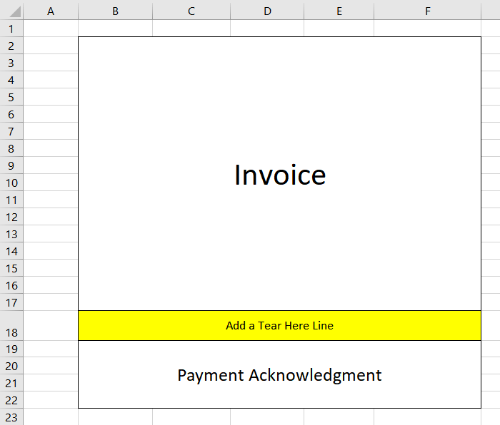
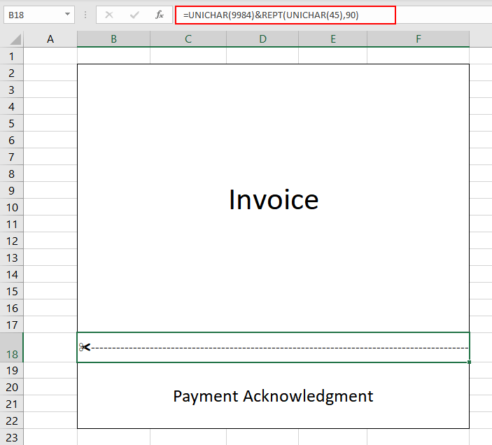
Now, the UNICHAR character code for scissors is 9984 to 9987, and we can choose any of them, while the Unicode character of the dash is 45. Using the UNICHAR and REPT functions, let's compile the Excel formula to make our 'Tear Here' line.

The ampersand sign (&) is used as a concatenation operator to join the results of UNICHAR and REPT functions. The REPT function is used to repeat the given text a given number of times. Here as per the width of our document, we chose to repeat the dash 90 times.

Example 2 – Creating a Rating System using UNICHAR Function

In this example, we are trying to create a rating system for all the famous museums in Amsterdam. Instead of the boring rating of 1-5, we will create an in-cell pictograph using the UNICHAR function where we can include star ratings and emoticons.

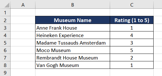
Based on the ratings in column C, we can use the REPT & UNICHAR functions to create a star rating pictograph in column D. The Excel formula will be as follows.

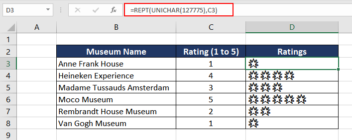
In the above formula, we are using the REPT function, where we are repeating the star symbol (UNICHAR(127775)) as per the rating. If the museum is rated 1 star, the star will be repeated once and so on.

Now, who doesn't love a few emojis? So, let's add emoticons using the UNICHAR function depicting the experience at each museum based on the ratings. A few references to the emojis in Unicode are as follows.

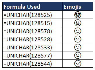
We can now add a few of these emoticons to make our rating system more presentable, along with the IF function. We will use a straightforward nested IF function that if the rating is 1, use one particular emoji; if the rating is 2, use another emoji, and so on.

The formula will be as follows.

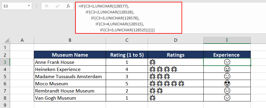
This looks much better on a mobile phone.

Note:

Instead of writing the above formula with the nested IF statements we can write it in a comparatively simpler way using IFS or SWITCH functions:

The logic is almost same for all the three formulas, the later two are just syntactically simpler than first one.

Example 3 – Sales Trend Report using the UNICHAR Function

Suppose your manager has given you a task to compile the total sales for each month. Now, this is your opportunity to make an excellent impression and make the Excel report impressive & presentable.

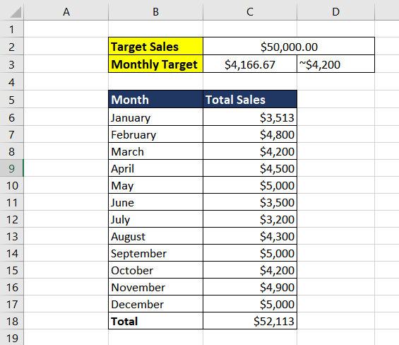
A basic sales report looks like this, including month-wise sales and the total sales made in a year.

To amp it up, let's use the UNICHAR function and showcase a sales trend along with the percentage by which we either missed the target or overachieved it. We will use arrow symbols to show if we are above or below the target.

UNICHAR(9660) returns (▲), an upward-facing triangle, which is also used to denote growth or an increase. UNICHAR(9660) returns (▼) which is a downward facing triangle/arrow that can be used to show a decline in trend or numbers. We will also use UNICHAR(9644), which returns( ▬ ). It is a simple dash that can denote no change in trend.

To begin with, we will build a simple logic that if our yearly target is $50,000.00, the monthly sales must be at least 50,000/12, which is $4,166.67. We must aim to achieve more, so we will take an upper round figure of $4200 sales each month.

Now, we will curate our Excel formula using a simple if and else logic.

IF(monthly sales is less than 4200), then (print downward arrow ▼), IF(monthly sales is more than 4200), then (print downward arrow ▲), else (print dash ▬)

Putting it all inside a formula:

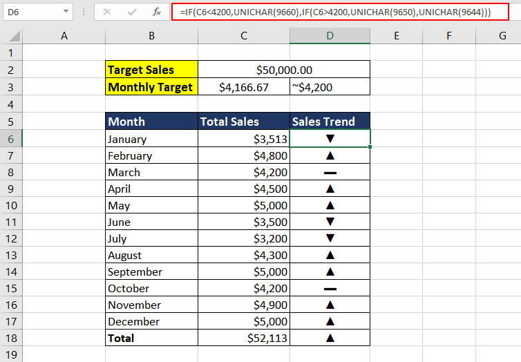
As we can see in the above example, months, where we didn't reach the sales target, show a downward arrow. In contrast, months like February and May show an upward arrow indicating overachieving the target. It already looks better.

We can go a step ahead and calculate the difference between the target and the actual sales. To calculate it in percentage, we will subtract the monthly target sales ($4200) from the actual sales, then divide it by 4200 and multiply by 100. To make it more presentable, we can join (concatenate) the symbol from column D and then add the percentage sign (%).

Compiling it in Excel form, the formula will be as follows:

Cell D6 is the character returned by the UNICHAR function. We combine that with the percentage difference and lastly add the percentage sign using the UNICHAR function. (The Unicode for (%) is 37). We have also used the basic ROUNDUP function to limit the decimal places to 2.

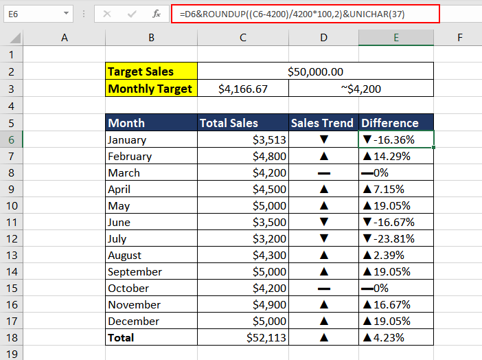
Looks pretty neat, right? For the total sales in cell E19, the difference will be calculated with the yearly target.

Example 4 – Creating Marketing Copies with Emojis

We have often seen a high usage of emojis and symbols in our app notifications, marketing emails, and advertisements. Marketers use them to deliver a better message, and they do look good. So, suppose you are into marketing and have to create one-liners for the brand.

In this example, we are creating marketing one-liners for a brand that sells smart bulbs.

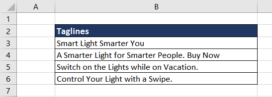
Now, the boss wants us to add emojis to these lines to amp it up. But how do we do that in Excel? Almost all emoticons we use on our phones are available in Excel using the UNICHAR function.

Join the text and the UNICHAR function using the ampersand (&) to concatenate the string as shown in the following image:

Example 5 – Remove Unnecessary Symbols

In this example, we have a few rudimentary English sentences that were reviewed, some of which were grammatically incorrect. So, the reviewer used tick (check mark) and cross symbols to indicate correct and incorrect sentences. We now wish to remove those symbols, so that we can send the sentences for correction.

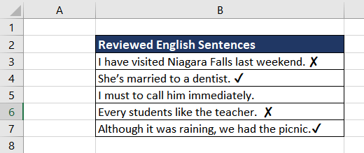
To remove the tick and cross symbols at the end of the strings, we can use UNICHAR, RIGHT, and LEFT functions. As there are two different symbols, we will use the IF function to check if the string ends with a tick mark or a cross mark.

The Unicode number for tick is 10004 and for cross it is 10008.

To check if the last character is tick or cross, we will use the RIGHT function.

The RIGHT function, when used without the second optional parameter, extracts the last character from the string.

Our final logic is going to be simple, take the last character from the string if it is either a tick or a cross then return the string with last character removed, otherwise return the string as is.

Compiling it in Excel form, the final formula will be as follows.

UNICHAR vs CHAR Function

As mentioned earlier, the CHAR function accepts numbers from 1 to 255. For additional character sets, we must use the UNICHAR function. For example, if we wish to use superscripts, subscripts, or special mathematical symbols, we will not be able to use the CHAR function.

In this example, we are trying to write the square root of 3 in the proper mathematical form.

One way to write it is in superscript or exponential form as 3^½, or in the radical form, it can be written as √3. The CHAR function has no such symbols, whereas the UNICHAR function can be used as follows.

The UNICHAR function is most convenient for characters that we cannot quickly access from the keyboard.

UNICHAR vs UNICODE Function

The UNICODE function is the opposite of the UNICHAR function. Now, we already know the functionality of the UNICHAR function, which returns the characters or symbols corresponding to the character code.

The UNICODE function returns the character code associated with the character. As both functions only accept one argument, the UNICHAR function returns the character code of the first character in the input text/string.

In this example, we can see that UNICHAR, with the input code number, returns the double arrow (⇼), whereas the UNICODE function with "⇼" as the input argument returns the corresponding Unicode number.

That was all about the UNICHAR function in Excel. We hope, we gave you a good grip on how it works. We will see you soon with another fantastic Excel function. Until then, keep crunching those numbers.