Excel UPPER Function – How To Use

Since Excel doesn't allow the inbuilt functionality of altering case types as Microsoft Word does, the UPPER function helps change the text to capital letters. All lowercase values are transformed to uppercase using the UPPER function. As it is a text function, the return value is always in text format.

Syntax

The syntax of the UPPER function contains a single argument and is as follows.

Arguments:

'text' – This is a mandatory argument. It is the input value that we want to convert to uppercase. The text argument can be a direct text or string in double quotes or a cell reference containing the value.

Important Characteristics of the UPPER Function

The notable features of the UPPER function are as follows:

• If the function's name or argument is incorrectly entered, Excel returns a #NAME error.
• The UPPER function converts the input number to text.
• When the text argument contains values with number formatting, the UPPER function removes the formatting in the return value.
• If the value of the text argument contains spaces or any special characters, the UPPER function does not affect them.

Examples of UPPER Function

The UPPER function provides a convenient and useful application, especially when dealing with large text data which requires a consistent case type. Let's understand the total utility of the function with the help of examples.

Example 1 – Plain Vanilla Version of UPPER Function

Here, we have taken a few sample data in lower and proper cases. We have also included an example of a string containing numbers and accented letters. Let's try using the UPPER function on them to understand its functionality better.

The formula used will be as follows.

As we can see, the first example was in proper case where the UPPER function changed all the lowercase letters to capital letters. Similar is the case in the second example. The third example is alphanumeric text, where the UPPER function changed the case type of all the letters while leaving the numbers unchanged. The fourth and last instance also confirms that the UPPER function works on accented letters changing its case type to uppercase.

Now that we have understood the basic functionality of the UPPER function, let's try and use it in a simple application.

Example 2 – Joining Text with UPPER Function

In this example, we asked people to submit their home addresses. As all the input fields were separate, the address was divided into columns for address, city, and state.

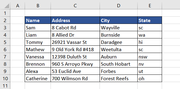
For the complete mailing address, we can simply combine the parts in columns C, D, and E using the TEXTJOIN function or ampersand symbol (&). But, the names of the states are in lowercase, whereas ideally, they should be in uppercase. So, using the UPPER function, we can capitalize the state's name and then combine it to form a complete address.

The formula used will be as follows.

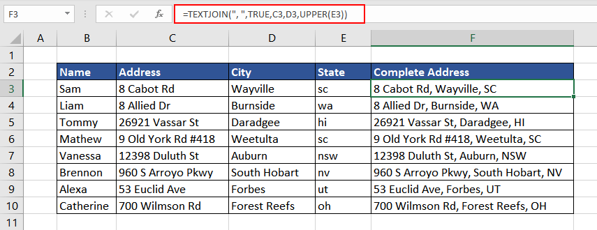
Now, the complete address can be used directly for mailing.

Example 3 – Converting Date into Uppercase

As mentioned, one of the characteristics of the UPPER function is that when used on Number Format values, the return value loses its formatting. So, if the UPPER function is used on dates, the return value is the number sequence as stored in Excel.

Then, how to convert dates in uppercase?

The solution is to use a combination of TEXT and UPPER functions. The TEXT function will first convert the value into text format and present it in the given date format. The UPPER function will then convert the return value of the TEXT function into uppercase.

The formula used will be as follows.

In his way, we can transform all values in number formats to uppercase in Excel.

Example 4 – Checking if Text is in Uppercase

In this instance, we have downloaded a list of acronyms and abbreviations from the web. We have to check and forward the list further. As they were downloaded, a few abbreviations are in lowercase which is neither correct nor presentable. Checking them manually would be time-consuming, so we will use the EXACT and UPPER functions instead.

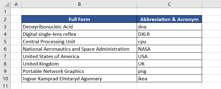
So, let's check if the short forms are in uppercase. The formula used will be as follows.

We first convert the value in column C to uppercase using the UPPER function and then make a case-sensitive comparison with the original value using the EXACT function.

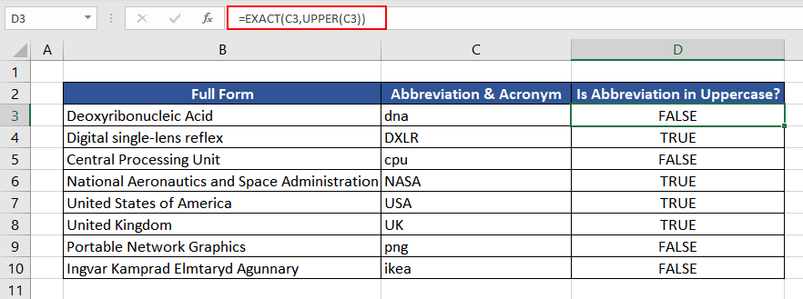
As we can see, many abbreviations and acronyms are not in capital letters, since the return value of the EXACT function is FALSE. To solve this, we can wrap up the EXACT and UPPER functions in a simple IF function to finally convert all the abbreviations to uppercase. The logic used will be as follows.

If the text in column C is in uppercase, then return the text as it otherwise, convert the text to uppercase and return it.

The formula used will be as follows:

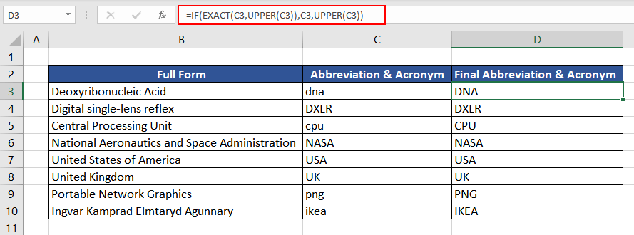
We now have the final data, which is both presentable and grammatically correct.

Example 5 – Using Data Validation with UPPER Function

Instead of checking the existing data for its case type, we can use the UPPER function along with the Data Validation option in Excel to compel the users to enter details only in uppercase. This way, the data collected will be in the correct case type.

In this instance, we are collecting the information in our guest book, which includes names, phone numbers, and remarks. The phone number and remarks can be in any case type, while we want all the names in uppercase for further data processing. We will apply Data Validation only in the cells that will carry the names.

First, select the cell and under the Data tab, choose the Data Validation option from Data Tools.

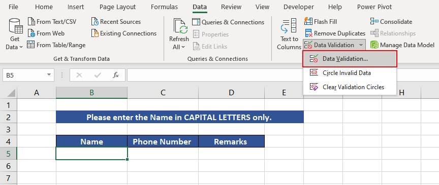
Once you select the Data validation option, a dialogue box pops up. In the Validation criteria, choose Custom.

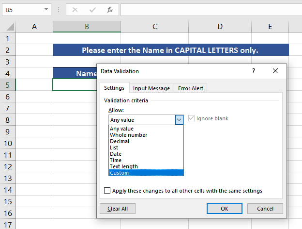
Now enter the UPPER function to be used in the Formula tab and Press OK. The formula used will be as follows.

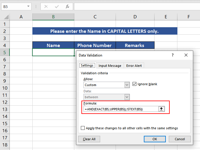
You are now all set. The Data Validation will automatically get activated as soon as the user enters data. Now, let's understand the logic behind the formula used.

The UPPER function first transforms the input value to uppercase. The EXACT function then compares the return value of the UPPER function with the input value to check if they are in the same case type, which is uppercase.

The second part of the formula using the ISTEXT function is an additional check of whether the input value is in text format. Combining both functions in the AND function, the Data Validation approves the input value only if both functions return the value TRUE. This means that only if the input value is text and is in capital letters will Excel accept the value.

If the input value does not meet these two conditions, Excel returns an error as a pop-up.

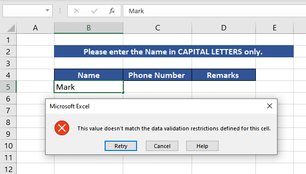
At the end of the day, all the data collected in the guest book will contain names only in uppercase.

LOWER vs. UPPER vs. PROPER Functions

There are other text functions, like the UPPER function, which help change the case type of the input value. The LOWER function modifies the case of the input value to lowercase, while the PROPER function capitalizes the initials of each word.

Here we have taken a famous quote as an input value for all three functions in cell C2.

As we can see, all three functions change the input value to the intended case type.

We hope you understood all there was about the UPPER function. Practice the UPPER function to discover more applications till we return with another intriguing and practical Excel function to make your data look more stunning and presentable.