Excel VALUE Function – How To Use

The VALUE function is a text function that converts a number from text format to numerical format where data is in an Excel-recognized format such as date, currency, time, etc. Mostly, if Excel recognizes a number, it automatically converts the data into numerical format. However, in other cases, we can do so using the VALUE function.

The VALUE function is most helpful when we seek compatibility with other spreadsheet programs and for using the numerical text resulting from text functions in calculations.

Excel VALUE Function

Syntax

The syntax of the VALUE function is quite straightforward and is given below.

=VALUE(text)

Arguments:

The VALUE function accepts only one argument, and it is mandatory.

'text'– This mandatory argument contains the value in text format that needs to be converted. The value of the text argument can be passed as a direct value in double quotes or as a cell reference.

Important Characteristics of the VALUE Function

Some noteworthy features of the VALUE function are as follows.

  • The VALUE function only accepts the value that is recognized by Microsoft Excel such as constant number, locale formatted number, date, or time. If the value of the text argument is any value that is not recognized by Excel, the function results in a #VALUE! error.
  • If the value of the text argument is empty, the VALUE function returns zero.

When using the VALUE function, it is important to note the alignment of the data as left-aligned data indicates text format whereas right-aligned data is number format.

Examples of VALUE Function

There are instances when the given data which looks like a number cannot be used further for calculations and analysis. In such scenarios, the VALUE function comes in very handy. Below are some examples to provide a better understanding of the function.

Example 1 – Simple Use of VALUE Function

In this example, we will use different types of input values for the text argument to better understand the functionality of the VALUE function.

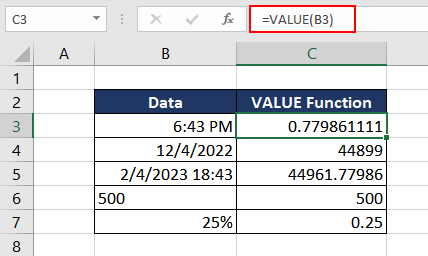
We have taken time, date, date and time together, number in text format, and percentage as the input values. The function used is as follows.

=VALUE(B3)
Simple Use of VALUE Function

In the first example, the value of the text argument is a time value which upon conversion to numerical format is transformed into the serial number. Excel stores time as fractions of a day. The VALUE function simply converted the time format to an actual serial number which can further be used in formulas.

The next example is in date format and like the time data, the VALUE function converts the date value to a sequential number as stored in Excel. The third example is a combination of date and time, and the VALUE function returns the expected result of the corresponding serial number and fraction of both date and time in cell C5.

The fourth example is a text which looks like a number. If we wish to use the data in cell B6 for any calculations, the result will also take on the text format. With the help of the VALUE function, the number is transformed from text format to numerical format.

The last example is a percentage value. The VALUE function returns the calculated numerical value of the percentage which is 0.25 in this case.

Now that the basic functionality of the VALUE function is clear, check some useful applications of the same in the examples below.

Example 2 – Converting String to Number using VALUE Function

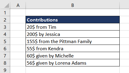
In this scenario, we collected small donations from our neighbors to get essentials for the homeless shelter. The data collected was user-generated hence it is in text format.
Converting String to Number using VALUE Function

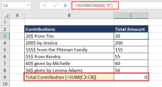
To calculate the total donations received, we can extract the dollar amount and then sum it up. To segregate the donation amount from the given text, we will use the TEXTBEFORE function. It will extract the characters that occur before the dollar sign ($), which is the amount in this case. The formula used is as follows.

=TEXTBEFORE(B3,"$")

Now that the donation amount is segregated in column C, the total donation can be calculated.
Converting String to Number using VALUE Function

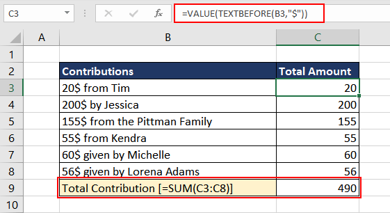
Unfortunately, all the extracted data in column C is text, which is clear due to its left alignment, since the TEXTBEFORE function is a text function. Therefore, the total sum couldn't be downloaded as seen in cell C10. To rectify this, we will use the VALUE function to convert all the data in column C into the numeric format and then calculate the total donation received. The updated formula to be used is as follows.

=VALUE(TEXTBEFORE(B3,"$"))
Converting String to Number using VALUE Function

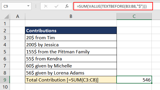
We can combine everything in one formula as follows.

=SUM(VALUE(TEXTBEFORE(B3:B8,"$")))
Converting String to Number using VALUE Function

Note: One can also use the LEFT function in place of the TEXTBEFORE function to achieve the same result.

Example 3 – Converting Currency to Numerical Format

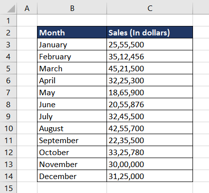
Here, in this case, we have received the monthly sales for the last year. As the sales report is from the India office, the currency formatting is different where a comma is used as a group separator in hundreds, thousands, and so on. Excel does not recognize the formatting, so it treats the sales numbers as text.
Converting Currency to Numerical Format

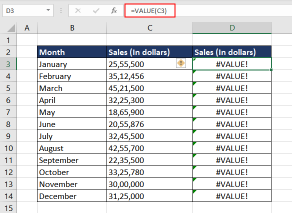
To be able to use the data for further calculations, we wish to convert them from text format to number format. As it is not an Excel-recognized format, the VALUE function will return a #VALUE! error.
Converting Currency to Numerical Format

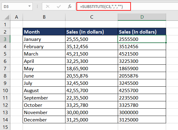
To overcome this, we can first use the SUBSTITUTE function to replace all the commas with an empty string and then use the VALUE function. The formula used will be as follows.

=SUBSTITUTE(C3,",","")
Converting Currency to Numerical Format

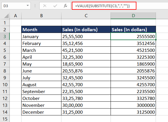
Now the sales values in column D are in a recognizable format i.e. text, with the help of the VALUE function, we can convert the same in number format. Combining both steps, the final formula used will be as follows.

=VALUE(SUBSTITUTE(C3,",",""))
Converting Currency to Numerical Format

As evident by the right alignment of the data in column D, all the sales values are now in a number format and therefore can be further used for calculations.

Example 4 – Converting Time using the VALUE Function

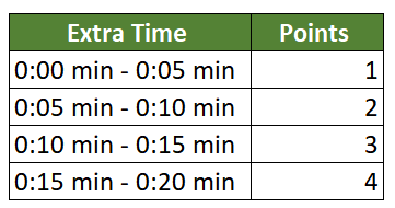
In this example, we are conducting an online test where the completion time is set to 10:00 AM. However, every applicant can take extra time up to 20 minutes, but points will be assigned depending on the extra time taken which will eventually be deducted from the actual score. Here are the points to be deducted as per the completion time.
<p>The VALUE function is a text function that converts a number from text format to numerical format where data is in an Excel-recognized format such as date, currency, time, etc. Mostly, if Excel recognizes a number, it automatically converts the data into numerical format. However, in other cases, we can do so using the VALUE function.</p> <p>The VALUE function is most helpful when we seek compatibility with other spreadsheet programs and for using the numerical text resulting from text functions in calculations.</p> <p><img class="aligncenter size-full wp-image-8529" src="https://exceltrick.com/wp-content/uploads/2023/02/Excel-VALUE-Function.png" alt="Excel VALUE Function" width="753" height="396" /></p> <h2>Syntax</h2> <p>The syntax of the VALUE function is quite straightforward and is given below.</p> <div class="excelFormula"><code><span class="operator">=</span><span class="function">VALUE</span>(text)</code></div> <p style="margin: 0px;"><strong>Arguments:</strong></p> <p>The VALUE function accepts only one argument, and it is mandatory.</p> <p style="padding-left: 30px;">'<em>text</em>'– This mandatory argument contains the value in text format that needs to be converted. The value of the <em>text </em>argument can be passed as a direct value in double quotes or as a cell reference.</p> <h2>Important Characteristics of the VALUE Function</h2> <p>Some noteworthy features of the VALUE function are as follows.</p> <ul> <li>The VALUE function only accepts the value that is recognized by Microsoft Excel such as constant number, locale formatted number, date, or time. If the value of the <em>text </em>argument is any value that is not recognized by Excel, the function results in a #VALUE! error.</li> <li>If the value of the <em>text </em>argument is empty, the VALUE function returns zero.</li> </ul> <p><span style="font-size: revert; color: initial;">When using the VALUE function, it is important to note the alignment of the data as left-aligned data indicates text format whereas right-aligned data is number format.</span></p> <h2>Examples of VALUE Function</h2> <p>There are instances when the given data which looks like a number cannot be used further for calculations and analysis. In such scenarios, the VALUE function comes in very handy. Below are some examples to provide a better understanding of the function.</p> <h3>Example 1 - Simple Use of VALUE Function</h3> <p>In this example, we will use different types of input values for the <em>text </em>argument to better understand the functionality of the VALUE function.</p> <p>We have taken time, date, date and time together, number in text format, and percentage as the input values. The function used is as follows.</p> <div class="excelFormula"><code><span class="operator">=</span><span class="function">VALUE</span>(B3)</code></div> <p><img class="aligncenter size-full wp-image-8530" src="https://exceltrick.com/wp-content/uploads/2023/02/value-function-in-excel_02.png" alt="Simple Use of VALUE Function" width="428" height="256" /></p> <p>In the first example, the value of the <em>text</em> argument is a time value which upon conversion to numerical format is transformed into the serial number. Excel stores time as fractions of a day. The VALUE function simply converted the time format to an actual serial number which can further be used in formulas.</p> <p>The next example is in date format and like the time data, the VALUE function converts the date value to a sequential number as stored in Excel. The third example is a combination of date and time, and the VALUE function returns the expected result of the corresponding serial number and fraction of both date and time in cell C5.</p> <p>The fourth example is a text which looks like a number. If we wish to use the data in cell B6 for any calculations, the result will also take on the text format. With the help of the VALUE function, the number is transformed from text format to numerical format.</p> <p>The last example is a percentage value. The VALUE function returns the calculated numerical value of the percentage which is 0.25 in this case.</p> <p>Now that the basic functionality of the VALUE function is clear, check some useful applications of the same in the examples below.</p> <h3>Example 2 - Converting String to Number using VALUE Function</h3> <p>In this scenario, we collected small donations from our neighbors to get essentials for the homeless shelter. The data collected was user-generated hence it is in text format.</p> <p><img class="aligncenter size-full wp-image-8531" src="https://exceltrick.com/wp-content/uploads/2023/02/value-function-in-excel_03.png" alt="Converting String to Number using VALUE Function" width="429" height="244" /></p> <p>To calculate the total donations received, we can extract the dollar amount and then sum it up. To segregate the donation amount from the given text, we will use the TEXTBEFORE function. It will extract the characters that occur before the dollar sign ($), which is the amount in this case. The formula used is as follows.</p> <div class="excelFormula"><code><span class="operator">=</span><span class="function">TEXTBEFORE</span>(B3,"<span class="string">$</span>")</code></div> <p>Now that the donation amount is segregated in column C, the total donation can be calculated.</p> <p><img class="aligncenter size-full wp-image-8532" src="https://exceltrick.com/wp-content/uploads/2023/02/value-function-in-excel_04.png" alt="Converting String to Number using VALUE Function" width="565" height="305" /></p> <p>Unfortunately, all the extracted data in column C is text, which is clear due to its left alignment, since the TEXTBEFORE function is a text function. Therefore, the total sum couldn't be downloaded as seen in cell C10. To rectify this, we will use the VALUE function to convert all the data in column C into the numeric format and then calculate the total donation received. The updated formula to be used is as follows.</p> <div class="excelFormula"><code><span class="operator">=</span><span class="function">VALUE</span>(<span class="function">TEXTBEFORE</span>(B3,"<span class="string">$</span>"))</code></div> <p><img class="aligncenter size-full wp-image-8533" src="https://exceltrick.com/wp-content/uploads/2023/02/value-function-in-excel_05.png" alt="Converting String to Number using VALUE Function" width="561" height="306" /></p> <p>We can combine everything in one formula as follows.</p> <div class="excelFormula"><code><span class="operator">=</span><span class="function">SUM</span>(<span class="function">VALUE</span>(<span class="function">TEXTBEFORE</span>(B3:B8,"<span class="string">$</span>")))</code></div> <p><img class="aligncenter size-full wp-image-8534" src="https://exceltrick.com/wp-content/uploads/2023/02/value-function-in-excel_06.png" alt="Converting String to Number using VALUE Function" width="545" height="307" /></p> <p><strong>Note:</strong> One can also use the <a href="mailto:https://exceltrick.com/functions/excel-left-function/">LEFT function</a> in place of the TEXTBEFORE function to achieve the same result.</p> <h3>Example 3 - Converting Currency to Numerical Format</h3> <p>Here, in this case, we have received the monthly sales for the last year. As the sales report is from the India office, the currency formatting is different where a comma is used as a group separator in hundreds, thousands, and so on. Excel does not recognize the formatting, so it treats the sales numbers as text.</p> <p><img class="aligncenter size-full wp-image-8535" src="https://exceltrick.com/wp-content/uploads/2023/02/value-function-in-excel_07.png" alt="Converting Currency to Numerical Format" width="418" height="387" /></p> <p>To be able to use the data for further calculations, we wish to convert them from text format to number format. As it is not an Excel-recognized format, the VALUE function will return a #VALUE! error.</p> <p><img class="aligncenter size-full wp-image-8536" src="https://exceltrick.com/wp-content/uploads/2023/02/value-function-in-excel_08.png" alt="Converting Currency to Numerical Format" width="584" height="426" /></p> <p>To overcome this, we can first use the <a href="mailto:https://exceltrick.com/functions/excel-substitute-function/">SUBSTITUTE function</a> to replace all the commas with an empty string and then use the VALUE function. The formula used will be as follows.</p> <div class="excelFormula"><code><span class="operator">=</span><span class="function">SUBSTITUTE</span>(C3,"<span class="string">,</span>","")</code></div> <p><img class="aligncenter size-full wp-image-8537" src="https://exceltrick.com/wp-content/uploads/2023/02/value-function-in-excel_09.png" alt="Converting Currency to Numerical Format" width="582" height="426" /></p> <p>Now the sales values in column D are in a recognizable format i.e. text, with the help of the VALUE function, we can convert the same in number format. Combining both steps, the final formula used will be as follows.</p> <div class="excelFormula"><code><span class="operator">=</span><span class="function">VALUE</span>(<span class="function">SUBSTITUTE</span>(C3,"<span class="string">,</span>",""))</code></div> <p><img class="aligncenter size-full wp-image-8538" src="https://exceltrick.com/wp-content/uploads/2023/02/value-function-in-excel_10.png" alt="Converting Currency to Numerical Format" width="585" height="426" /></p> <p>As evident by the right alignment of the data in column D, all the sales values are now in a number format and therefore can be further used for calculations.</p> <h3>Example 4 - Converting Time using the VALUE Function</h3> <p>In this example, we are conducting an online test where the completion time is set to 10:00 AM. However, every applicant can take extra time up to 20 minutes, but points will be assigned depending on the extra time taken which will eventually be deducted from the actual score. Here are the points to be deducted as per the completion time.</p> <p><img 11></p> <p>As the first step, we will calculate the extra time taken in each case. The formula used will be as follows.</p> <div class="excelFormula"><code><span class="operator">=</span>B4<span class="operator">-</span>$C$2</code></div> <p><img 12></p> <p>Now that we have all the values in column C, we can use the <a href=":https://exceltrick.com/functions/excel-nested-if/">nested IF function</a> to compare the time as per the point system and then assign the corresponding points. However, while using the delayed time data from C4:C7, we will wrap it in the VALUE function to ensure that Excel treats the time value as a number and not text.</p> <p>The logic used will be as follows.</p> <p>If the delayed time (C4) is less than 5 minutes, then assign 1 point, else if the delayed time is less than 10 minutes, assign 2 points….) and so on till 20 minutes. If no condition is met, the formula returns FALSE.</p> <p>The formula used will be as follows.</p> <div class="excelFormula"><code><span class="operator">=</span><span class="function">IF</span>(C4<span class="operator"><</span><span class="function">VALUE</span>("<span class="string">0:05</span>"),1,<span class="function">IF</span>(C4<span class="operator"><</span><span class="function">VALUE</span>("<span class="string">0:10</span>"),2,<span class="function">IF</span>(C4<span class="operator"><</span><span class="function">VALUE</span>("<span class="string">0:15</span>"),3,<span class="function">IF</span>(C4<span class="operator"><</span><span class="function">VALUE</span>("<span class="string">0:20</span>"),4))))</code></div> <p><img 13></p> <p>Now we have the final points that will be deducted from the final score in each case. With the help of the VALUE function, we were able to convert the time value from minutes to numerical format and execute the nested IF function.</p> <h2>VALUE Function vs NUMBERVALUE Function</h2> <p>Both the VALUE and NUMBERVALUE functions convert text that looks like a number from text format to numerical format but the <a href="mailto:https://exceltrick.com/functions/excel-numbervalue-function/">NUMBERVALUE function</a> transforms the data using the given group and decimal separators which help the function understand the format.</p> <p>If the data is not in an Excel-recognized format, the VALUE function returns a #VALUE! error whereas with the NUMBERVALUE function, we can mention the group and decimal separator used in the data to convert it. Let's understand it better using an example.</p> <p><img 14></p> <p>The data in cell B4 is a currency value in euros and is in a text format. The VALUE function does not recognize the data and hence throws a #VALUE! error whereas the NUMBERVALUE function converts the data from text to number format due to the mentioned decimal and group separator.</p> <h2>VALUE Function vs VALUETOTEXT Function</h2> <p>Now we know that the VALUE function converts text that looks like a number from the text format to numerical format. The VALUETOTEXT function performs the opposite conversion. The VALUETOTEXT function converts a value to text format depending on the concise or strict format.</p> <p>Hopefully, now you have a clear idea about how to use the VALUE function to your advantage. Practice and discover new applications of the said function.</p>

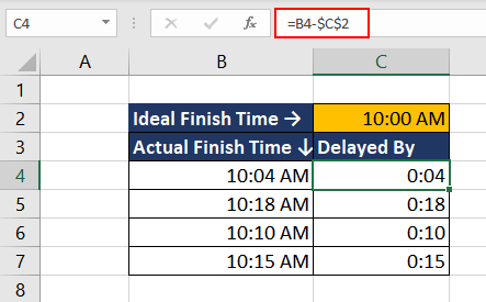
As the first step, we will calculate the extra time taken in each case. The formula used will be as follows.

=B4-$C$2
Converting Time using the VALUE Function

Now that we have all the values in column C, we can use the nested IF function to compare the time as per the point system and then assign the corresponding points. However, while using the delayed time data from C4:C7, we will wrap it in the VALUE function to ensure that Excel treats the time value as a number and not text.

The logic used will be as follows.

If the delayed time (C4) is less than 5 minutes, then assign 1 point, else if the delayed time is less than 10 minutes, assign 2 points….) and so on till 20 minutes. If no condition is met, the formula returns FALSE.

The formula used will be as follows.

=IF(C4<VALUE("0:05"),1,IF(C4<VALUE("0:10"),2,IF(C4<VALUE("0:15"),3,IF(C4<VALUE("0:20"),4))))
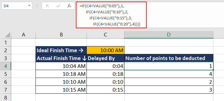
Converting Time using the VALUE Function

Now we have the final points that will be deducted from the final score in each case. With the help of the VALUE function, we were able to convert the time value from minutes to numerical format and execute the nested IF function.

VALUE Function vs NUMBERVALUE Function

Both the VALUE and NUMBERVALUE functions convert text that looks like a number from text format to numerical format but the NUMBERVALUE function transforms the data using the given group and decimal separators which help the function understand the format.

If the data is not in an Excel-recognized format, the VALUE function returns a #VALUE! error whereas with the NUMBERVALUE function, we can mention the group and decimal separator used in the data to convert it. Let's understand it better using an example.

VALUE Function vs NUMBERVALUE Function

The data in cell B4 is a currency value in euros and is in a text format. The VALUE function does not recognize the data and hence throws a #VALUE! error whereas the NUMBERVALUE function converts the data from text to number format due to the mentioned decimal and group separator.

VALUE Function vs VALUETOTEXT Function

Now we know that the VALUE function converts text that looks like a number from the text format to numerical format. The VALUETOTEXT function performs the opposite conversion. The VALUETOTEXT function converts a value to text format depending on the concise or strict format.

Hopefully, now you have a clear idea about how to use the VALUE function to your advantage. Practice and discover new applications of the said function.

About Shubhra Jain

Meet Shubhra Anand Jain, a dedicated Excel enthusiast with over 5 years of expertise, specializing in data analysis, complex formula development, and automation. Based in Sweden, she's on a mission to simplify Excel, one formula at a time. Check out Shubhra's extended profile here.