The YEAR function in Excel is categorized as a Date/Time function. It extracts the year component from a valid, Excel recognized date and returns it as a four-digit value. For instance, when a cell contains the date 12/25/2001, the YEAR function returns 2001.
The YEAR function is used by financial analysts for extracting the year component from dates for grouping transactions in a given year. The YEAR function can also be nested inside the DATE function to relay the extracted year to the DATE function.

Syntax
The syntax of the YEAR function is as follows:
=YEAR(serial_number)Arguments:
'serial_number ' – This is a required argument where you will need to add the serial number for the date or a cell reference to a cell containing such date, from which you want to extract the year component.
Important Characteristics of the YEAR function
- The value supplied to the serial_number argument must be a valid date (i.e., a serial number that Excel recognizes as a date or a date returned from another function).
- If the supplied value is a text string, the YEAR function will return a #VALUE error.
Examples of YEAR Function
A few examples should clear up any confusion regarding the YEAR function. Let's take a look.
Example 1 – Plain Vanilla Formula for the YEAR Function
Before we venture into the deeper end of the pool, let's start with some basic formulas. We'll use the bare-bones formula for the YEAR function to extract the year component of date like so:
=YEAR(A2) //Year From Date
=YEAR(A3) //Year From Serial Number
=YEAR("10-Jul-2008") //Year From Date as String

In the image, notice how the cell reference to cell A2 may also be replaced with several other values to extract the year component of a date. The formula accepts a cell reference containing the date or serial number, or you could directly supply a valid date as a text string inside the formula, too.
Example 2 – YEAR Function with TODAY and DATE Function
The YEAR function is often used with two other functions, the TODAY and DATE functions. In our example, we'll use all of these together to understand how each function feeds values to the other function. Let's assume we want the first day of the current year as the output. We will use the following formula:
=DATE(YEAR(TODAY()), 1, 1)
Let's walk through the mechanics of this formula. The TODAY function, as we know, returns today's date. The TODAY function, therefore, relays today's date to the YEAR function.
The YEAR function extracts the year component from the value relayed by the TODAY function, which will be the current year.
Subsequently, the YEAR function relays the value to the DATE function. The other two arguments of the DATE function have already been entered as 1 and 1, which represent the month and day components, respectively.
The final output, of course, will be January 1, 2021 – the first day of the current year. If you see a number instead of a date as your output, make sure that you've formatted the cell as a date.
Example 3 – Get nth Day of the Year
Let's say you want to make some quick computations for your investment returns and you need the number of days you were invested in an asset during this calendar year. To do this, we'll use a combination of the DATE and YEAR functions.
Before we get to the formula, though, it's important to know about an important characteristic of the DATE function. When you enter 1 in the month argument and 0 in the day argument, the DATE function returns the last day of the year preceding the year entered in the year argument. If this sounds confusing, consider the following formula:
=DATE(2001, 1, 0) //Returns December 31, 2000In this case, the DATE function will return December 31, 2000.
Alright, now that you're aware of this feature of the DATE function, let's use this to compute the nth day of the year.
The formula we will use is:
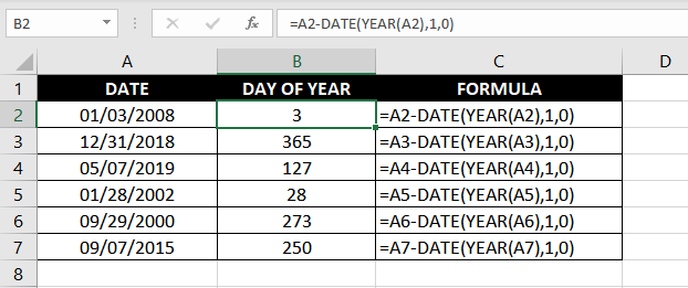
=A2 - DATE(YEAR(A2),1,0)
Let's break this formula down and see how it works. The YEAR function extracts the year component from the date in cell A2 and relays it to the DATE function. The DATE function, then, returns the last day of the previous year since we have entered the month argument as 1 and the day argument as 0. Therefore, the DATE function returns December 31, 2007.
The date in cell A2 is January 03, 2008. Excel stores dates as serial numbers, and therefore, it will subtract the serial number for December 31, 2007, from January 03, 2008. The difference will give us the nth day of the year. In our example, it's the 3rd day. Similarly, the nth day is calculated for all the dates in the range.
We could also slightly tweak the above formula to get the corresponding day of the year for today's date. In that case, the formula will look like so:
=TODAY() - DATE(YEAR(TODAY()),1,0)Example 4 – Get the Fiscal Year from a Date
Let's say we want to extract the fiscal year from a list of dates. The fiscal year, also known as the financial year, is denoted by the year in which the last month occurs. For instance, assuming that a fiscal year starts on April 1 and ends on March 31, and we're looking at the period between April 1, 2001, and March 31, 2002, the fiscal year will be 2002.
To get the fiscal year from a date, we'll use the following formula:
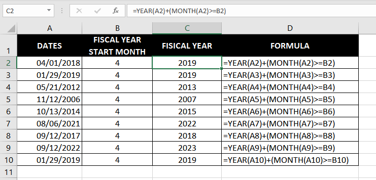
=YEAR(A2) + (MONTH(A2) >= B2)
Let's disassemble the formula and understand it – one function at a time. We'll first discuss the part of the formula that occurs after the + sign. The MONTH function fetches the month component from the date in cell A2, which in the first instance is 4 (i.e., April). If this number is greater than or equal to (>=) the value in cell B2, it will return TRUE. If not, it will return FALSE.
The YEAR function simply extracts the YEAR component from the date in cell A2. Next, if the 2nd half of the formula (i.e., part after the + sign) has returned TRUE, it will add 1 to the year returned by the YEAR function, and 0 otherwise.
In the first case, since April (4) is greater than or equal to the start month of the fiscal year (4), 1 has been added to the year 2018 and our final output is 2019. However, as in the second instance, the date in cell A3 is January 29, 2019, so the extra 1 does not get added to the year part (because 1 is not greater than or equal to 4) and hence the formula has returned the year as it is.
Example 5 – Get Percent of Year Complete
You're a big saver and an even bigger investor. You love playing with numbers and you're curious about running some digits to assess the performance of your investments. You made a lot of investments on January 1, 2001. You sold a few of these during the year. Now, you need the percent of year that you held these investments for so you can weigh the returns by their holding period.
This is the formula we will use to compute the percent of the year complete:
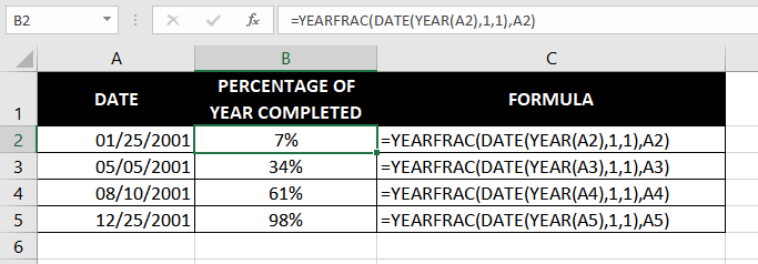
=YEARFRAC(DATE(YEAR(A2), 1, 1), A2)
Let's start with the DATE function. The YEAR function nested inside the DATE function extracts the year component from the date in cell A2 and relays it to the DATE function. The other two arguments represent the month and day components, respectively, and both these arguments have been supplied the value '1'. This essentially means that the DATE function will return the first day of the year extracted by the YEAR function.
The DATE function then relays this value to the YEARFRAC function. The relayed value is supplied to the YEARFRAC function's start_date argument and the value in cell A2 is supplied as the end_date argument. The YEARFRAC function then computes the difference in terms of the number of days between the two dates and divides it by the total number of days in a year to give us the final output.
The final output, therefore, in our example is 7%, 34%, 61%, and 98%.
You can now pat yourself on the back and rightfully claim to be an expert on the YEAR function. While you solidify your expertise with some practice, we'll go put together another tutorial with some nifty formulas to help you become an undefeated Excel champion.


