The YEARFRAC function is categorized as a Date and Time function in Excel. It returns the difference between two supplied dates in terms of years. When the difference is fractional, the output will have a non-integer output, such as 3.5 years, for instance.
Fractional years can save a lot of time for financial analysts projecting revenues or cash flows since it gives them the flexibility to simply use the output of the YEARFRAC function for making relevant computations.

Syntax
The syntax of the YEARFRAC function is as follows:
=YEARFRAC(start_date, end_date, [basis])Arguments:
'start_date' – This is a required argument where you need to supply the date from which you want the calculation to begin.
'end_date' – This is a required argument where you supply the date that represents the end of the calculation period.
'basis' – This is an optional argument that controls how days are counted while computing fractional years (as per the table below).
Various Possible Values of 'basis'
| 'basis' value | Calculation | Convention |
|---|---|---|
| 0 (default) | 30 days per month / 360 days per year | US Convention |
| 1 | Actual days / Actual of days in the year | – |
| 2 | Actual days / 360 days per year | – |
| 3 | Actual days / 365 days per year | – |
| 4 | 30 days per month / 360 days per year | European Convention |
Important Characteristics of the YEARFRAC Function
- The YEARFRAC function includes both the start_date and the end_date in its calculations.
- If the basis argument consists of a value less than 0 or greater than 4, the YEARFRAC function returns a #NUM error.
- If the date(s) supplied in either or both of the start_date or end_date arguments is invalid, or if the value supplied in the [basis] argument is non-numeric, the YEARFRAC function returns a #VALUE error.
Examples of YEARFRAC Function
Let's try to see some examples of the YEARFRAC function.
Example 1 – Plain Vanilla Formula for the YEARFRAC Function
Let's play around with some dates, shall we? We'll start slow to understand the mechanics of the YEARFRAC function's formula. Here's the formula we'll use:
=YEARFRAC(A2, B2)
The example is pretty straightforward. We have two dates 13 months away from each other. When we apply the YEARFRAC function, it views the difference in terms of years. Let's verify this, though.
A difference of 13 months is more than 1 year and less than 2 years. The first 12 months account for 1 full year. The remaining 1 month (or 30 days based on the default US convention) is translated by Excel into years as 30/360, which is 0.083. This is what the YEARFRAC function returns – 1.083 years (i.e., 1 + 0.083).
Example 2 – Changing 'basis' in the YEARFRAC formula
Let's see how changing the 'basis' argument affects the output of the YEARFRAC function. Let's assign a value of 1 to the 'basis' argument like so:
=YEARFRAC(A2, B2, 1)
The default value of the 'basis' argument is 0, where the difference is calculated assuming 30 days a month and 360 days a year. When we assign a value of 1 to the 'basis' argument, the formula doesn't make these assumptions. Instead, it looks at the actual number of days for all the months considered in the calculation.
In our example, notice how the output changes to 1.085 from 1.083 that we computed previously. This is because it computes the actual number of days between the dates and divides it by 365 to calculate the final output.
So, it calculates a year up to December 25, 2002, as 365 days and adds the remaining 31 days, i.e., 6 remaining days of December and 25 days of January. The total difference between the dates in terms of days is, therefore, 396 days. Dividing this by 365 gives us our final output, 1.085 years.
Okay, that takes care of all the basics we need to look at. Let's move to the deeper end of the pool and take a jab at some bulkier formulas.
Example 3 – Calculate the Percentage of Year Complete
We can use a combination of the YEAR, DATE, and YEARFRAC functions to calculate how much of a certain year has passed on a given date in terms of percentage. The formula isn't all the complex once you see what we're trying to do, though. Here's the formula we'll use:
=YEARFRAC(DATE(YEAR(A2), 1, 1), A2)
Let's use March 31, 2001, so we can verify the output. We know that when March ends, we're through with a quarter of the year, which means 25% of the year has passed.
Alright, let's disassemble the formula now. We'll start from the inner-most function – the YEAR function. The YEAR function simply extracts the year component of a date. In this case, the YEAR function extracts the year component from the date in cell A2 and relays it to the DATE function.
The DATE function's purpose in this formula is simply to set the YEARFRAC function's start_date to the first day of the year as per the date in cell A2. In our example, the YEAR function will relay the year 2001 to the DATE function. Consequently, the DATE function returns January 1, 2001, and relays it to the YEARFRAC function.
The YEARFRAC function's start_date argument now has its value set to January 1, 2001. Next, we reference cell A2 in the end_date argument. Essentially, the formula will make the calculations for the period between the first day of the year based on the date in cell A2 and the date in cell A2 itself. Evidently, things check out – our output is 0.25 (or 25%). You could even go ahead and format the cell as a percentage to display the output as 25%.
Example 4 – Calculate Age Using the YEARFRAC Function
Let's suppose you run a small successful company. For a company to be successful it has to treat its employees well. And as a part of our employee wellness initiative, we like to enroll our employees in a 4-week free post-retirement planning session during their last two years with us (only 58+ employees are eligible). This makes the transition easier for them.
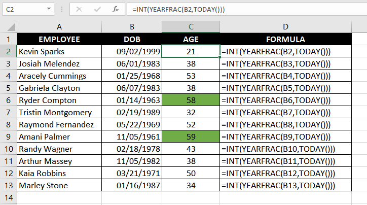
Now, instead of investing in expensive software, we requested our receptionist to maintain a spreadsheet for us. The spreadsheet contains all employee’s names with their birthdays. We let Excel formulas take care of the remaining part. So, here's the formula we'll use to calculate an employee's age:
=INT(YEARFRAC(B2, TODAY())
The formula calculates the difference between the employee's birthday and today's date. Next, the value is relayed to the INT function. All that the INT function does is truncate the value and convert it into an integer.
Now, we have the age of all employees. It's easy to find employees with the age of 58 and above. But what if your company had 100s of employees? You'd want something more convenient, eh?
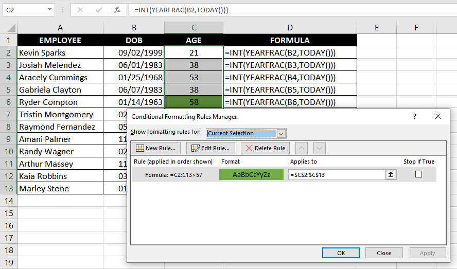
Let's use conditional formatting to color those cells where output is 58 or above with the color green. Head over the Styles section in the Home tab of your Excel sheet and click on New Rule. Under the Select a Rule Type section, select the last option Use a formula to determine which cells to format. Next, insert the following formula in the Edit the Rule Description section:
=C2:D13 > 57Next, click on the Format button and navigate to the Fill tab. Choose the color green (or any other color of your choice), and press OK. Press OK again and you should now see the Conditional Formatting Rules Manager. Make sure the Applies To field has the appropriate range selected — in our case, it should be =$C$2:$C$13.

When you're done, you'll see your soon-to-retire employees' age light up in green.
Recommended Reading – How To Calculate Age In Excel
Example 5 – Using IF Function and YEARFRAC function
What we'll accomplish with the IF function here is similar to what we did with conditional formatting. However, it never hurts to have an extra tool or two at your disposal, right?
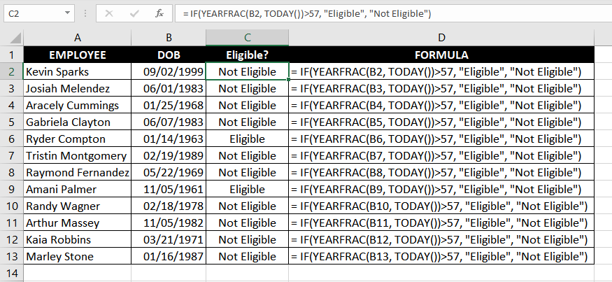
Okay, so let's say we were to identify employees that are going to retire in less than 2 years using the IF and YEARFRAC function. Here's the formula we can use:
=IF(YEARFRAC(B2, TODAY())>57, "Eligible", "Not Eligible")
We'll use the same data in this example so we can verify that both methods accomplish the same purpose. When we apply the formula, notice how two rows return the string "Eligible" while others return "Not Eligible". And voila — this checks out with the output we had in our previous example.
We're through with the YEARFRAC function, but we promise not to take too long before coming back with another function that you can add to your Excel toolkit. Meanwhile, play around with the YEARFRAC function and keep your number-crunching spirits strong.


