How to Calculate Years of Service in Excel (2 Easy Ways)

Finding out the years of service of employees may come with their resignation. The intent may be to find out the employment duration or to use that duration to determine/calculate some form of entitlement. If resignation is not the case, you may be trying to figure out the years in service of the current employees.

Working towards calculating the years of service in Excel, we have this tutorial comprised of simple and customizable methods. We'll be dealing with the YEARFRAC, DATEDIF and EDATE functions with help from the INT and TODAY functions and the & operator to make our formulas better applicable to our example case. Speaking of that, let's have a look at the example.

Recommended Reading: How to Calculate Age in Excel

Example

We'll keep it super-duper simple. This is the example we will use to calculate the years of service in Excel:

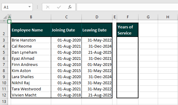
We have a small extract from a mock-up employees' database. The joining dates of 10 employees are in column C with the dates of their last working day in column D. The objective is to find the years of service which will be the difference between the joining and leaving dates. Ready to roll with the numbers?

Let's get calculating!

Method #1 – Using YEARFRAC Function

Let's start with the non-elusive one (you'll see what we mean in the next section). Using the YEARFRAC function, we can arrive at the years of service between two dates. The two dates make the start date and the end date. YEARFRAC calculates the number of whole days between the dates and returns it as a year fraction. E.g. if there are 182 days between the dates, YEARFRAC will return 0.5.

Now let's apply the YEARFRAC function to our example for calculating years of service and see the results. Below is the formula:

Beginning with the main function, YEARFRAC takes the date in cell C3 as the start date and the one in D3 as the end date. The YEARFRAC function is to calculate the years between these two days according to the selected basis. The basis will be listed in the Formula AutoComplete as the parameters are entered:

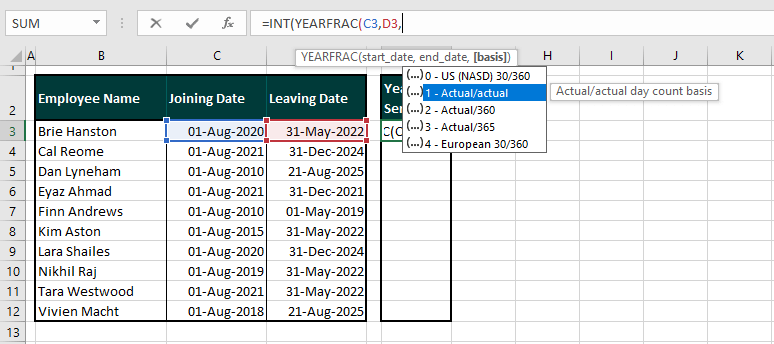
Instead of using an assumed number, we will go with the actual/actual basis so that the real days between the two dates can be counted i.e. months with 30 and 31 days will be rightly counted and so will leap years.

You can stop the formula right there and you will have the service years returned in decimal. But if we take it a step further and add the INT function, we can get the value as an integer. Of course you can leave out the INT function and simply decrease the decimal places to 0 but that would round the answer to the nearest whole year.

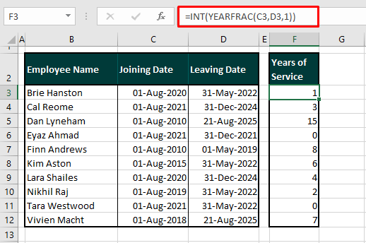
By using the INT function, we round the number down to the nearest integer. That will give us only the complete years in service. E.g. in the first instance of our case example, the fraction returned from YEARFRAC alone was 1.83 which has been rounded down to 1 by the INT function. Here is our whole example case with the YEARFRAC and INT functions:

If you want to add text to the results (e.g. 1 year), you can use any of the concatenating functions and formulas. Actually, we'll show you how to do just that. Keep reading!

Method #2 – Using DATEDIF Function

If the matter is of calculating a period between two dates, the DATEDIF function serves that exact purpose. The DATEDIF function measures the difference between two provided dates and returns the difference in years, months, days, or a selection from all three based on the entered code. We have detailed the formulas for finding:

• only the years,
• the years and months,
• the years, months, and days.

We said something about elusivity earlier. It's important to know how to enter the syntax correctly because Excel's Formula AutoComplete has no log of DATEDIF as it is an undocumented function. Now let's see how to get it right.

Calculating Only Years

This is how to use the DATEDIF function to return the difference between two dates in years:

The joining date and leaving date have been given to the DATEDIF function as the start date and end date. Now DATEDIF needs to return the difference between the dates in C3 and D3 in years. To achieve that, the code supplied in the formula is "y" for years.

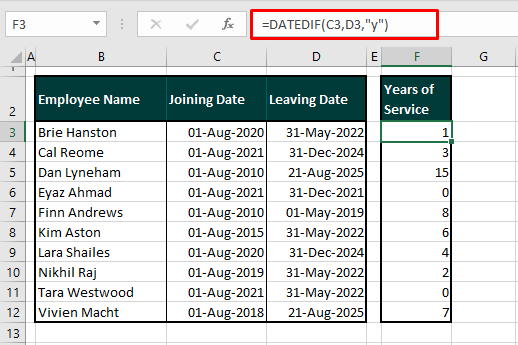
Note: If the result is 0, the implication is that the duration was not a complete year. For such instances, you can choose to set the IF function to return a custom text string instead of 0. See the example below:

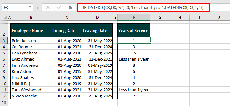
This might look like pantomime but it is just the formula used earlier wrapped in the IF function. If DATEDIF's result equals 0, then the text string "Less than 1 year" should be returned. If not, then DATEDIF's result is to be returned. In row 3, the years of service was 1 which has been returned as it is. In row 6, the result was 0 hence, the IF function has returned the custom text "Less than 1 year".

Calculating Only Years & Months

Just the whole number of years for some cases doesn't show the complete picture and the number of months may also be required for a clearer representation of the duration. We will show you how to use the DATEDIF function to return the months between two dates.

As per your requirement, you can have the number of years and the months calculated in separate columns. We will take on a single formula to have the years and months in the same column, distinguished by the text "Y" for years and "M" for months. Let's have a look at the formula:

Firstly, we have DATEDIF for returning the number of years between the two dates, and then the & operator joins the text "Y" to DATEDIF's result. In the first instance, the output from this part of the formula will be 1Y.

Then, we have used DATEDIF again pretty much the same way to return the number of months but the code has been changed to "ym". If you're asking why you can't use "m" for months as "y" for years, that's a good question. You could use "m" in the formula but it would return the total number of months. "ym" returns the number of months independent from the number of whole years. E.g. in the first instance, the service years have been calculated as 1 year and 9 months. Using "m" as the code would have returned 21 months.

After DATEDIF, the text "M" has been combined with the outcome with the & operator to return the result as 1Y 9M. To add the space character between the year and months, make sure you add a space in the formula at the end of the first text string or the beginning of the second text string. If you look carefully, you can see in the formula that there is a space character after Y making the text string "Y " otherwise the result would be 1Y9M.

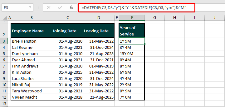
You can add your text string of choice for the years and months instead of "Y" and "M".

DATEDIF with IF Function

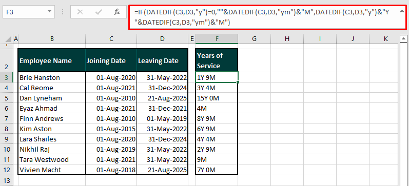
Here's a little bonus tip for you. Run a quick look over the previous example again and you'll see that a couple of differences between the dates are of less than a year. Let's take row 6 for analysis; the result of the difference between C6 and D6 is 0Y 4M. We can again use the IF function to return just the months for such a case. We have pieced together the formula below:

In this pseudo pantomime no. 2, we have taken the previously used formula and shuffled things around a little with the IF function to get just the months if the duration is less than a year. In the formula, if the difference in years equals 0, then the IF function will only return the months. If not so, then IF will return the years and months. Put like that, it's so simple, right?

Calculating Years, Months & Days

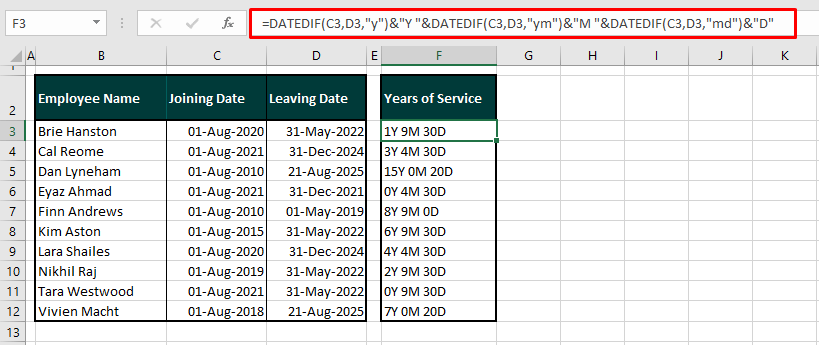
For certain calculations, you are going to need the details down specifically to the days in service. In order to get that, the period will have to be calculated in years, months and days. Using the DATEDIF function, we will compute the years, months, and days along with the & operator to differentiate the results. Let's dive into the following formula:

For the service duration, we have already gone through calculating the years and months with DATEDIF. Now we have used the same concept to add DATEDIF for the third time in the formula to return the number of days. With help of the & operator, we have connected DATEDIF with the code "md" to return the number of days independent of the complete years and months.

With the & operator, "D" has been added to the formula to indicate the days. Taking up the first instance, the formula has returned 1Y 9M 30D.

Service Duration till Current Date

As a scenario, you could be computing the years of service up until the current date. All you need to do is incorporate the TODAY function. The TODAY function returns the current date. Using the TODAY function in place of the end date will dynamically result in the duration up to the current date. Right up, we can show you an example of how you can use the TODAY function in such a way:

Suppose today's date is the 1^st of August 2025. If you look at the example case, we've swiped out the leaving dates in column D. In the formula, D3 has been replaced with the TODAY function which is without a parameter. This is the only change we have made to the formula from the previous section and it has resulted in the formula considering the end date as 01-08-2025. Now we have the following computations:

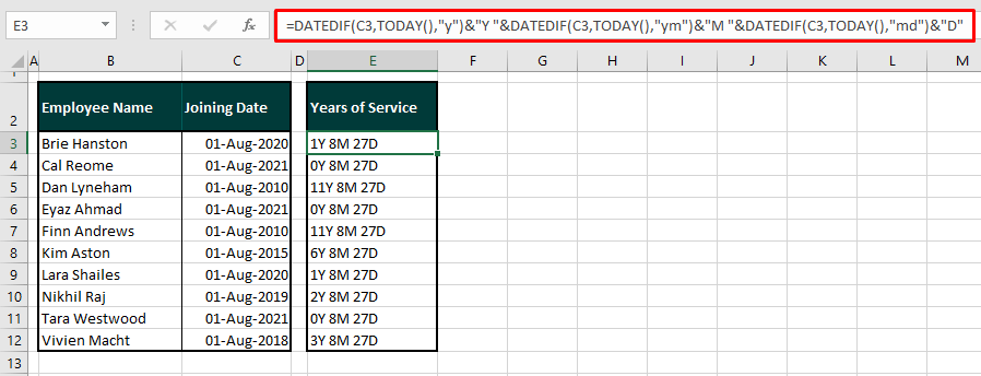
Note: Good news is that the TODAY function works dynamically as it is a volatile function; the values will recalculate with changes made to the worksheet. If the date has progressed since the previous change was made, the results will automatically be adjusted accordingly.

Service Duration after Fixed Number of Years

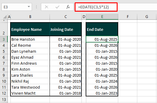
If you're comparing the performance of the employees after a certain duration of service, you need to add years to the start date. One way of doing this is through the EDATE function. The EDATE function returns the serial number of the date which is the given number of months after the start date. The months can be adjusted as years for them to be added. Here's the formula:

To arrive at the date 5 years from the joining date of an employee, we have entered the number 5 as the second argument in the formula. The number 5 alone would add months which is why we have multiplied 5 by 12 so that years are added instead. In this way, 5 years are added to the date in C3, taking the date from 01-Aug-2020 to 01-Aug-2025.

And that's that! By now we're hoping you got a decent footing on the grounds of calculating years of service in Excel. Wasn't it interesting to find some of the tips and tricks? We had a good time putting them together for you. What's that again? More Excel tricks? At your service!