How to Convert Negative Numbers to Positive in Excel

There are some very basic tasks that you would think Excel has it all covered with a single click. But sometimes what is basic to you and us, isn’t basic to Excel or maybe Excel expects us to apply one of many easy Excel tricks.

If you’re facing a spreadsheet, you are more likely to encounter many types of numbers and we see no one-click method of making positive numbers negative and negative numbers positive. That gives us the topic for the day; how to convert a negative number to positive in Excel.

We can think of 6 easy ways that do not involve doing it all manually: multiplying with minus one using a formula or Paste Special, using the ABS function, Flash Fill, a Custom Format, and VBA. We can quickly get down to the first method after we’ve seen the example we’ll be referring to for this tutorial.

Example

For our example case, we have a list of negative numbers which were copied from a database defining various discounts for each range of shopping points e.g. 10001-10500 points earn a 5% discount. Whilst separating the values of each range, we have ended up with the upper limit being copied like so:

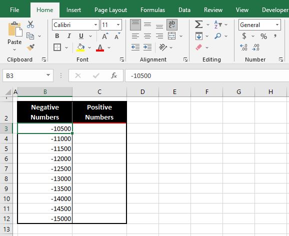
The upper limit was copied with the hyphens which have resulted in negative values for us. For calculations, we would prefer to remove the minus signs from all the numbers. But what if copy-pasting from the database was even more incompatible?

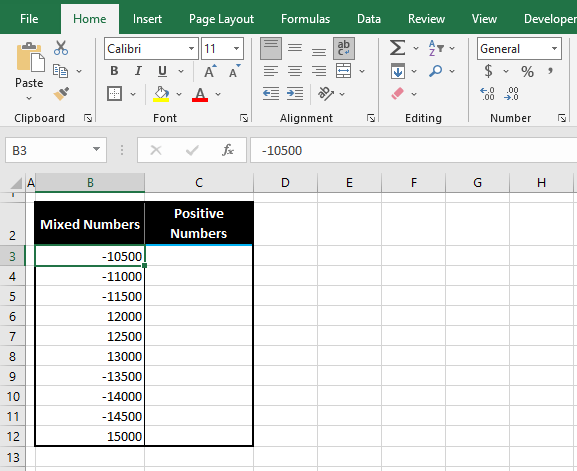
Now we have some numbers with the minus sign and some without. How should we deal with these? It’s all doable so…..

Let’s get converting!

Oh and here’s one more thing. All the methods in this guide can do with slight tweaking to convert positive numbers to negative. You just need the minus sign or a minus one at the right place!

Method #1 – Using ABS Function

 Works for mixed and negative numbers

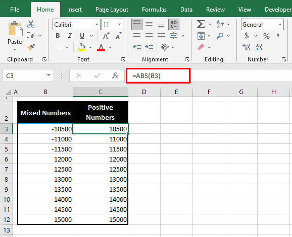
 Let’s get rolling with the first method. We will first try the ABS function in Excel to convert the negative numbers to positive numbers. The ABS function returns the absolute value of a number without its sign, whether positive or negative. Isn’t that just what we’re looking for? Let’s test it with this simple formula:

The ABS function takes a single argument to return a number without its sign. Our first value ready for conversion is in cell B3 and the ABS function changes -10500 to 10500.

This also works for positive numbers because the ABS function disregards the number’s sign and returns the absolute value of the number. Below we can see how the ABS function has worked for our list of mixed numbers.

Cue conversion:

Method #2 – Multiply by -1

Works only for negative numbers

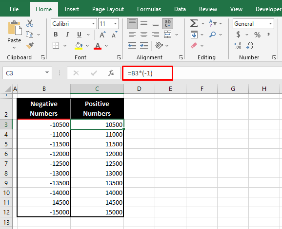
If you need to change a bunch of negative numbers into positive values, another option is to multiply them by -1. A little memory jogging down to secondary school math should remind how positive and negative signs work together. Jog back down to the application of this simple arithmetic formula to change negative numbers to positive:

The negative number in B3 is multiplied by -1. The two negative signs cancel each other out and then the value is multiplied by 1. This returns the number without the minus sign. It works the same for all negative numbers:

Why won’t this trick work for mixed numbers? It kind of will but it will reverse all the signs; the negative values will become positive and the positive values will become negative. And then you’ll be left with another trick to apply to work on mixed numbers. It only makes sense to use another method in the first place instead of trying to make this one work for both signs.

Method #3 – Multiply by -1 Using Paste Special

Works only for negative numbers

There’s another way to use the multiplying by -1 trick to make negative numbers positive. In the previous method, we used -1 in a formula. Now we will use it as a cell value, copy the value and use the Paste Special options to multiply it to the negative numbers. That’s the idea. And the demonstration is in the steps below:

• If you want to retain the original values, copy the numbers to another column, as we have done below. If not, you can overwrite the original values.
• Enter the value “-1” in any nearby empty cell.
• Copy that cell with the Ctrl + C

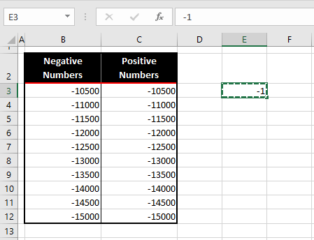
• Select the negative numbers you want to convert.
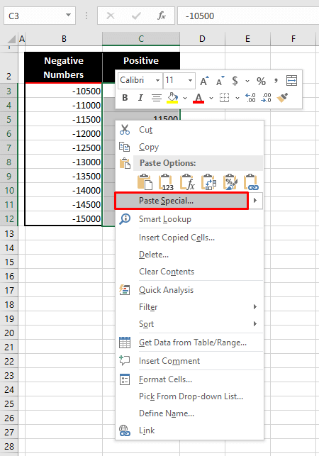
• Right-click on the selection and select Paste Special from the context menu to launch the Paste Special dialog box.
• You can also use the Alt + E + S keys to do this.

• In the dialog box, select the Multiply radio button from the Operation

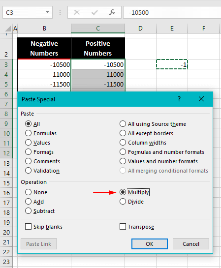
• Then select the OK command button.
• The negative numbers will be multiplied by -1 and the minus signs will be removed:

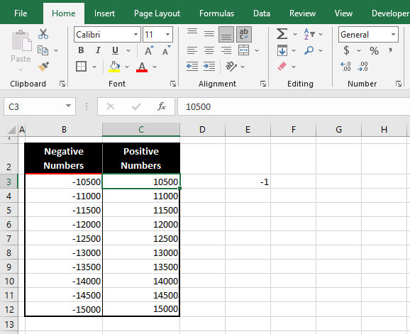
• Delete the cell with the -1 value if you are done converting number signs.

Note: The complete keyboard shortcut for this method after copying -1 and selecting the target cells is:

Alt + E + S + M + Enter

Method #4 – Using Flash Fill

Works for mixed and negative numbers

Another fairly quick method of converting negative values to positive ones is to use Flash Fill. Flash Fill is like an Excel copycat. The Flash Fill feature automatically fills values after you have entered one or two as an example.

Flash Fill will work fine for mixed numbers as it will pick up on the pattern of returning the numbers without the minus sign. Read more on this in the footnotes of this section. Time to put Flash Fill to the test with our example:

• In the column next to the numbers, manually enter the first value without a minus sign to provide an example for Flash Fill.

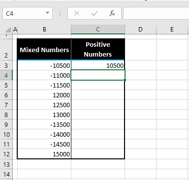
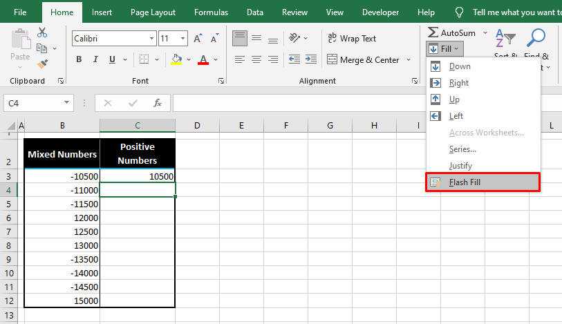
• With any one of the target cells selected, from the Home tab, select the Fill button in the Editing Then select Flash Fill from the menu to activate the feature.
• Alternatively, use the Ctrl + E keys to use Flash Fill.

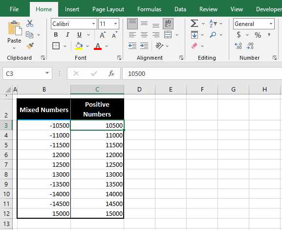
Voila copycat! Flash Fill will fill the target cells with the numbers sans the minus signs:

Notes:

You must make sure that the first value in your mixed numbers is a negative value. Otherwise, you will have to continue to provide examples until you reach a negative value in order to provide a pattern for Flash Fill to pick. But still, you need not worry if the first value in your data is positive; you can simply change it by adding a minus sign and then you’re good to go.

Our examples above consist of 5-digit numbers. Flash Fill will also work for mixed digit numbers. E.g. if you have a mix of 2-digit and 3-digit numbers, Flash Fill will correctly return the numbers without the minus sign.

Method #5 – Using Custom Format

Works for mixed and negative numbers

Applying a custom format will display the negative numbers as positive numbers. That’s right; the numbers will not be converted, only displayed as positive because they will be formatted. You may prefer this method when you need the numbers to be deducted in a formula but want them to be displayed without the minus sign (although you could just add a minus sign in the formula).

A custom format will work for displaying mixed and negative numbers as positive values because it will change the way the numbers appear as per one format. Let’s apply one to our example with these steps:

We are copying the original numbers to another column for comparison and will format the new column. You may overwrite the original column with the new format.

• Select the numbers you want to format.

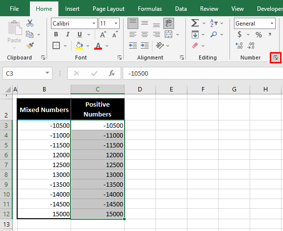
• Click on the dialog launcher of the Number group in the Home tab to access the Format Cells dialog box or press the Ctrl + 1
• The Number tab of the Format Cells dialog box will show you the current format of the selected cells.

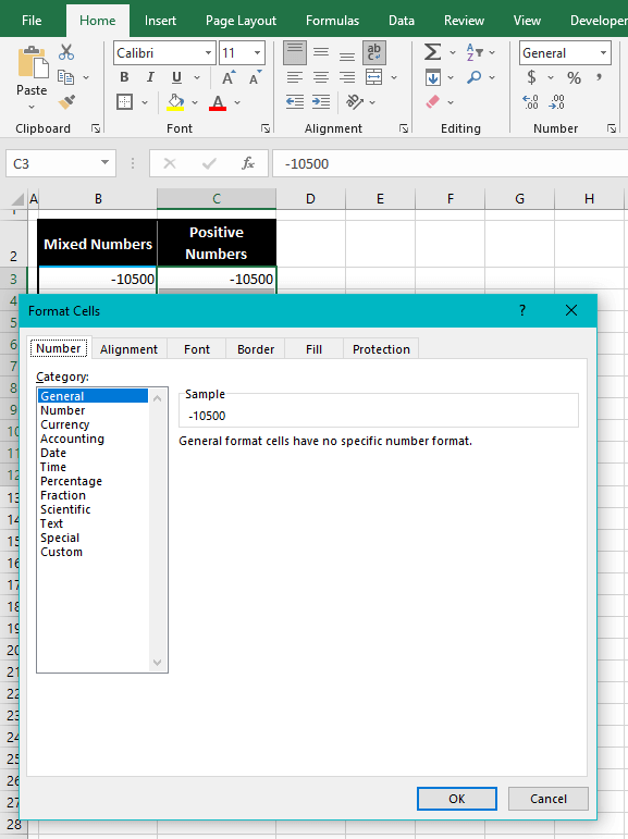
• Click on the Custom category from the pane and enter the following formatting code in the Type field:

• A sample will be displayed of the typed format:

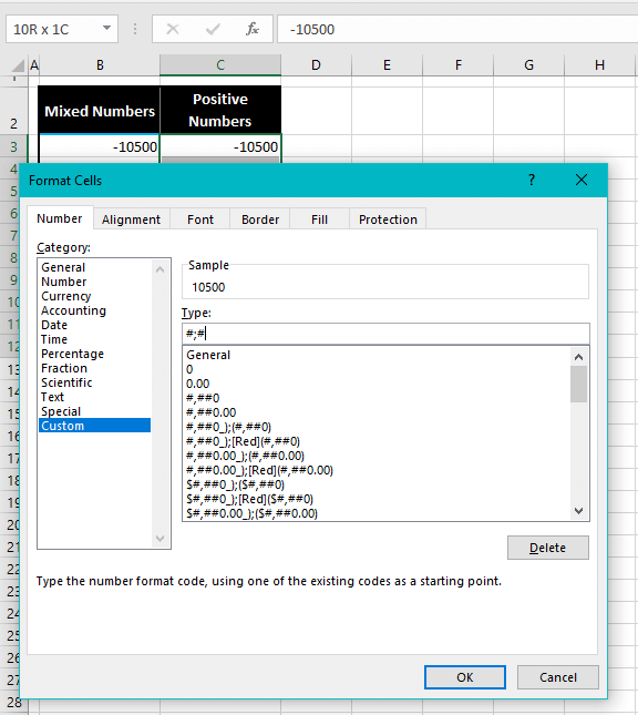
• Click on the OK button to close the dialog box.

The format will be applied to the selected cells and will be displayed in the Number Format bar.

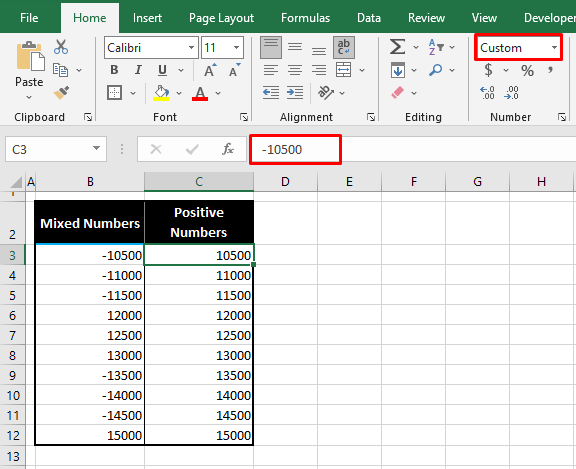
Selecting any of the formatted cells, the Formula Bar will display the actual value of the number, whether negative or positive.

Notes:

This formatting code will work for numbers with varying digits.

For numbers with thousands separators or decimals, you will need to edit the code to accommodate the desired format.

Method #6 – Using VBA

 Works for mixed and negative numbers

 For the code freaks, we have our final method of converting negative values to positive using VBA. VBA can be used to automate tasks in Excel with user-defined codes. Our code will use the IF function to check the negative values and convert them to positive ones. This is why it will work for converting mixed and negative numbers. We have the detailed steps for this here:

For explaining our case example, we have copied the numbers to a new column to show you the conversion. According to your requirement, you can choose to use the original values to convert.

However, with VBA, there is no undoing, and you cannot undo the task run by the code. It is therefore advisable to copy the data to a new column or to save the file before you run the code and close the unsaved file if you want to undo the macro.

• Select the cells with the numbers.
• Go to the Developer tab > Code group > Visual Basic icon to launch the VB
• In case you don’t have the Developer tab added to the ribbon, you can use the Alt + F11 keys.

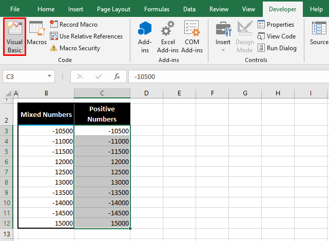
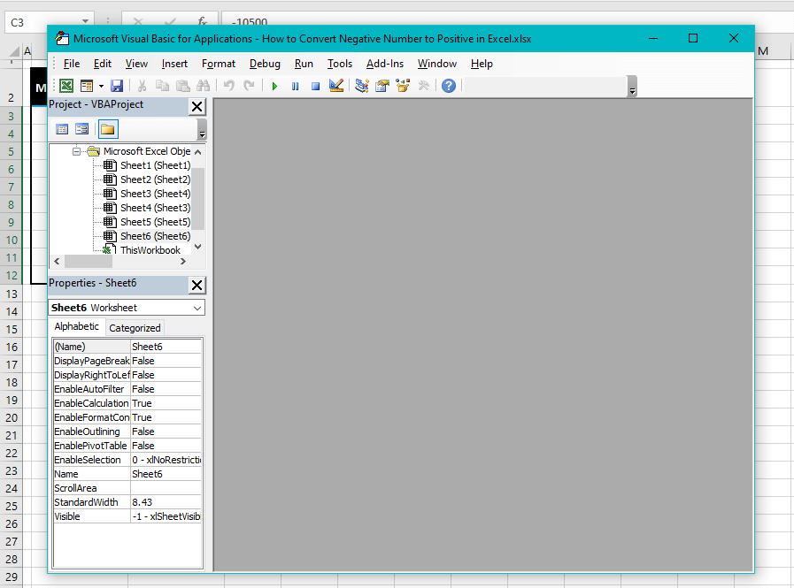
• The VB editor will be opened:

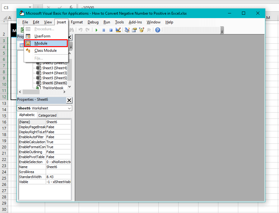
• Click on the Insert tab and select the Module option from the menu.

• This will open a Module window:

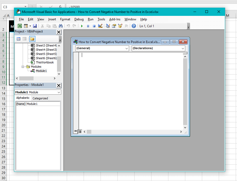
• Copy and paste the following code in the Module window to create a macro:

Sub MakePositive()
Dim ws As Worksheet
Dim rng As Range
Dim result As Range
Set ws = Application.ActiveSheet
Set rng = Application.Selection
For Each cell In rng
 If cell.Value < 0 Then
 cell.Value = cell.Value * -1
 End If
Next
End Sub

This code involves IF function to check each selected cell’s value to be less than 0, which implies that it would be a negative number. In case of a negative number, the value will be multiplied by -1 to eliminate the minus sign, returning the number as a positive value. The positive values in the selection would remain so.

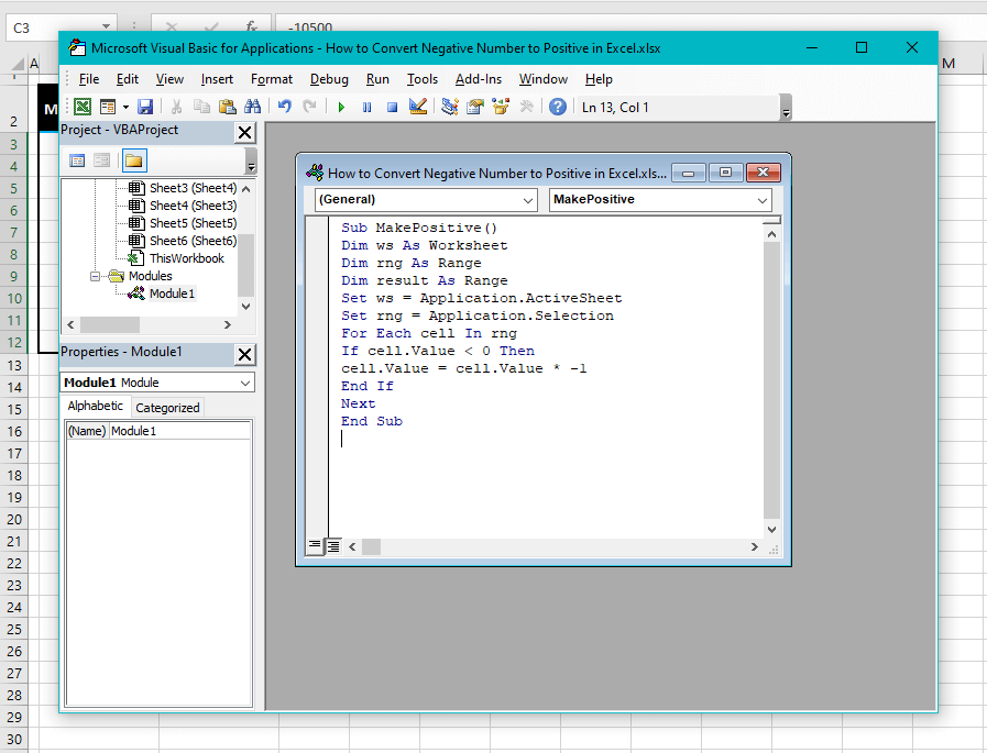
If you close the VB editor, the macro can be run later from the Developer tab or the View tab by clicking on the Macros icon and selecting the relevant macro from the list. To run the macro right away:

• After pasting the code in the Module window, press the F5

This runs the code and converts the negative numbers to positive from the selected cells:

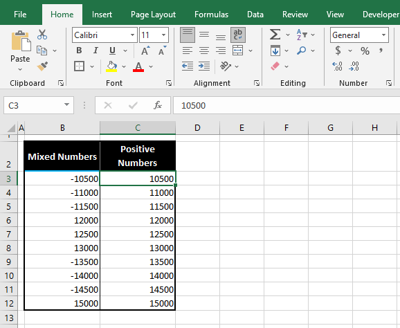
It’s a wrap! Those were 6 easy methods giving you a bucketful of options on how you want to go about converting the negative numbers on hand to positive ones.

Whether your numbers are all negative, mixed with positive, have varying digits, there’s more than one method to tackle them so that your mission is accomplished. We’re on a mission to bend more Excel culprits into submission. You’ll have us back in no time!