How to Extract Month from Date in Excel (5 Easy Ways)

With endless streams of data, we keep bouncing back to the same thing; organizing. Because data needs to be discernable and that requires displaying or sorting data differently. Dates may need to be split into days, months, or years for the associated analysis and we're focusing on one chunk of that for now.

In this tutorial, you will see a few ways on how to extract and display the month from a full date. Those ways use the TEXT, MONTH, CHOOSE and SWITCH functions and a custom date format. The methods are simple and explained thoroughly and you can pick one as per your Excel state of affairs.

Your options are the month in text (e.g. January, Jan, or custom), number (1 or 01), or display form (with the date value still intact). Therefore…..

Let’s get extracting! (No pain dental or otherwise.)

Method #1 – Using TEXT Function

The first method is simple, plain, and effective and is overlooked by the TEXT function. This function can be used to extract the month from a date in Excel. The TEXT function takes a value and converts it to text in the given number format. As to why we're talking about a value being text and a number format in the same go, you'll see in a while how the two meld together.

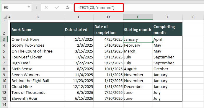
In this tutorial, we will use an example of the start and completion dates of writing a children’s book series. As a once-over, it would be helpful seeing what months the dates fall on. See this formula below and use it to extract the month from a full date using the TEXT function:

The TEXT function here is using the date in C3 and the format for the text is given by us as “mmmm”. This is the format code for the full month name. We have copied the formula down and across for the start and completion dates; these are the results for us:

In the formula, apply a different number format code enclosed in double quotes for the preferred output:

• m – returns the month number in a single digit (1 for January and 12 for December).
• mm – returns the month number in double digits (01 for January and 12 for December).
• mmm – returns the initial 3 letters of the month name (Jan for January and Dec for December).
• mmmm – returns the month name in full (January for January).

Bonus: Calendar/Fiscal Quarters

Where would we be without a small Excel trick in the balance? Out of balance? Keeping all in equilibrium, this is a little detail you can add to the data; the quarter of the year the month falls in. Use a formula like so to attach the related quarter with the month extracted from the date:

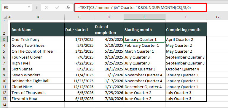
The first part of the formula is the TEXT function, picked straight out as it was used earlier. The second part is the text "Quarter" added with a leading and trailing space by the & operator.

The third part, also joined using the & operator, is the quarter number calculated by the MONTH and ROUNDUP functions. The MONTH function takes the month from the date in C3, i.e. 1. In the formula, we divide this number by 3 (1/3 equals 0.33) and use the ROUNDUP function to round the resulting number up to the nearest integer (0.33 rounds up to the number 1).

This number defines what quarter the month in the date falls in. That completes the formula and all the results are shown here:

Now you can see that the month function should be quite useful in this tutorial, and it is. We’ll explore a few more ways with the MONTH function for extracting months from dates. Let’s go into what the function itself can do.

Recommended Reading: How to Extract Year from Date

Method #2 – Using MONTH Function

In the preceding section, the month name was returned. Now this method we’re about to see returns the number of the month instead of the month name from a date. This is done with the MONTH function in Excel. The MONTH function on its own picks the month from a date and results in the month number (from 1 to 12, sequentially for the 12 months).

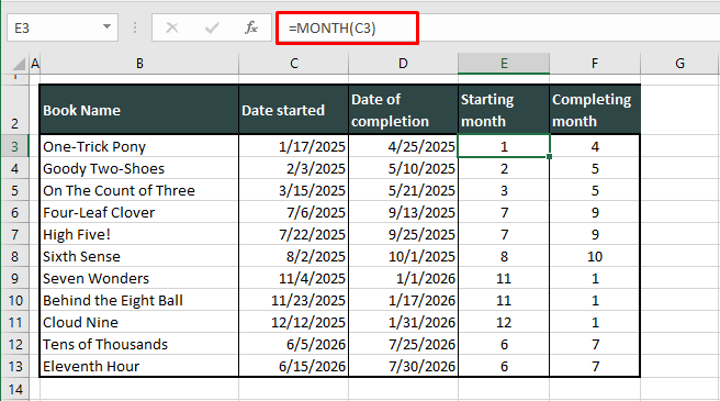
With this simple formula, you can get the month number from the date in C3:

The MONTH function will only need a date to sift out the month and return the month number:

Method #3 – Using MONTH Function with CHOOSE

Life comes with many difficult decisions and sometimes making a choice is the hardest thing. But in Excel, when you have it all mapped out, the CHOOSE function has it all figured out. The CHOOSE function takes an index number and returns a value set against that number. Therefore, it can be incorporated with the MONTH function to extract the month from a date and then return the month name.

Hold on, haven’t we done that already? And the CHOOSE function would also require listing all the twelve values down so why is it even useful here when there are simpler ways and shorter formulas to get the month name?

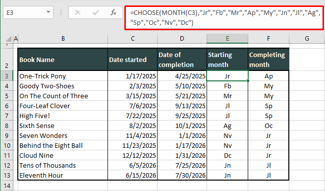
Suppose we want to assign codes to our book collection and a part of that code is 2 letters of the start month and 2 letters of the completion month, we would want the month names from the dates in 2 letters. So, we’ll abbreviate the month names (e.g. Jr for January, Fb for February) and use the following formula:

All the abbreviated month names have been typed out in order in the formula. This readies the CHOOSE function to pick out the month and display it when it gets the index number. The index number is brought about by the MONTH function in our example case. the MONTH function takes C3’s date and picks the month out as 1. This index number is passed to the CHOOSE function and it returns the first value lined up in the formula i.e. Jr.

The formula goes on that way e.g. with the date in D8, the month number comes out as 10. Against the number 10, the value in the formula is Oc which is displayed in F8.

You know what that also means? It means that if you accidentally get the order of the months wrong, the results will be misleading and you wouldn't even be aware. Excel gasp. There can be one way around this and it’s right around the corner. Actually it’s right ahead. Read below. 

Recommended Reading: How to Convert Date to Month and Year in Excel

Method #4 – Using MONTH Function with SWITCH

Now let’s switch things up a little. What a call that is, we are talking about the SWITCH function and how it can be used to pull the month from a date in Excel. Yes, we already know that can be done but what we're trying to avoid here is the lineup problems that come with the CHOOSE function.

The SWITCH function, much like CHOOSE, evaluates a value (e.g. a3) against a list of values (from a1 to a12) and returns its corresponding value (returns b3 against a3). So the first yay with the SWITCH function is that the values can be placed in any order, unlike the CHOOSE function.

The second yay is that in case there’s no matching value, an added default value will be returned. The nay is that all the values and their corresponding values will have to be listed in the formula (though this may be a yay point where the values will not be as straightforward as 1, 2, 3 and will have to be defined anyway).

Here is how the formula rolls out with the SWITCH and MONTH functions for extracting months from dates:

The difference from the CHOOSE function is quickly notable here; not only are the abbreviated months listed but also the values that they correspond to; the numbers. You can also see that the order is not important here as we have listed July first in the formula but what is important is getting the corresponding values right.

Again, the MONTH function will return the month number from the date in C3 and the SWITCH function will pull out the corresponding value from the formula and we will end up with “Jr” as the result.

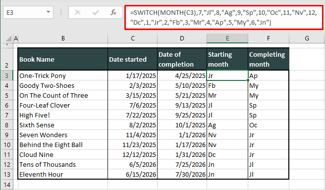
Hence, the final upside of using the SWITCH or the CHOOSE function is that you can get either function to deliver custom values for the months. If this is not your requirement, go with the TEXT function. You can also have the cell display the month but still be usable as a date but you’re going to have to read ahead.

Method #5 – Using Custom Date Format

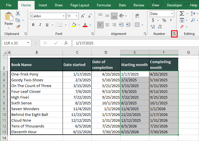
If your requirement isn’t as quirky as what you just saw, we have another way to get the month of a date to show. Use a Custom date format to make the name of the month appear instead of the date. If you’re okay with overwriting the data, use the format on the original data containing the dates. Otherwise, copy-paste the dates to the target column and apply the format there. The steps below will show you what to do to get the months from the dates after copy-pasting the dates to separate columns:

• Select the dates where you want the month names instead.
• Then click on the Number dialog launcher in the Home
• 
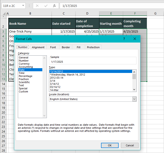
• The Format Cells dialog box will open with the Number tab and you will see the current format of the selected cells.
• 
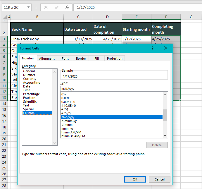
• Click on the Custom category from the left panel. This will also show you the formatting code for the current format.
• 
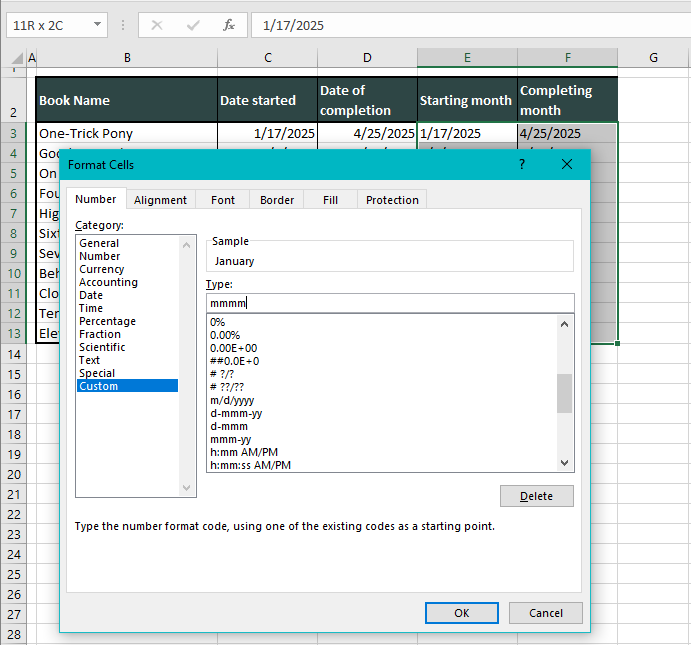
• Change the formatting code by entering the relevant format in the Type
• For the full month name, enter mmmm. For more formatting codes related to the month name and number, refer back to the earlier section on using the TEXT function.
• 
• When done, click on the OK

The dates in the selected cells will be formatted to just the month names.

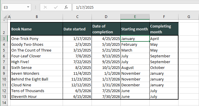
Note that the month names are only a display as the cells have been formatted. The original value is still the full date which can be confirmed by selecting any cell; you will see the date in the Formula Bar.

Since the original value is still a date, it can be used regularly in formulas and calculations as any date would.

We hope you’re Excel-updated on how to get the month from a date with some of the simple ways and Excel tricks shown in this tutorial. We also hope that this guide has pulled you into some sightseeing around here because if you look at it our way, Excel is a maze and we’re here with all the right cheat codes. You won’t get lost, give it a try!