This tutorial covers generating random numbers in Excel. Using the RAND, RANDBETWEEN and RANDARRAY functions, and VBA, we will demonstrate how to generate random whole numbers and decimals. We’ve also got you covered on generating random numbers without repeat values.
Why is randomizing important? Randomizing gives a fair and equal chance of selection to all units. For picking out a student or employee based on their role number or employee code, for picking lottery tickets, to set a random order, statistical analysis. All these examples require random number selections.
Excel hands us many ways of generating random numbers, some easy ones we’ll share with you today.
Let’s get generating! (Or randomizing! Or numbering!)
Method #1 – Using RAND Function
The RAND function returns a random decimal between 0 and 1. It is a volatile function and the numbers are recalculated every time the worksheet is recalculated.
As mentioned, the RAND function will return decimals, not integers but will generate random numbers nonetheless. Here’s the formula to use the RAND function to generate random decimals between 0 and 1:
=RAND()The RAND function is singularly entered without any arguments and instantly returns a random decimal. The Fill Handle can then be used to copy the formula and have as many random numbers generated as needed.
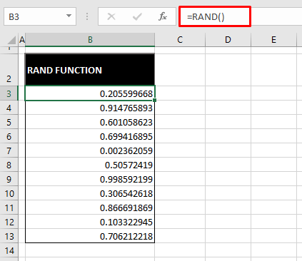
Since RAND is a volatile function, you will have to copy-paste the values to keep the values in place.
Given the many digits of these decimals, the RAND function is highly likely to return unique numbers.
A small addition to the RAND function can get RAND to generate random integers, or at least display them as integers. Let’s get a set of random numbers with this formula:
=RAND()*11+1The syntax becomes:
=RAND()*(b-a)+a
//b – Maximum number to generate
//a – Minimum number to generate
11 comes from deducting the minimum value from the maximum value. Since we want random numbers between 1 and 12, 12-1=11. Then the minimum value is added at the end of the formula.
If you want to include your minimum and maximum values in the generations, add 1 to your maximum value and subtract 1 from your minimum value.
The following are the results of this formula:
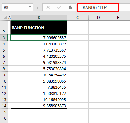
Now using the Decrease Decimal button in the Home tab’s Number group, reduce the decimals until you are left with integers.
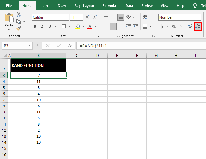
The ROUND function can be used (instead of decreasing decimals) with this formula to deliver integers.
On its own for generating random numbers, it might not be what you’re looking for. Paired with other functions, it can generate random integers with and without repetitions. We have a couple of examples ahead.
Method #2 – Using RANDBETWEEN Function
The RANDBETWEEN function returns a random number between the two numbers you specify. The very first thing to note about RANDBETWEEN is that it will generate repeat values. Let’s say we want 12 random numbers from the sequence of 1 to 12, this is the formula we will use:
=RANDBETWEEN(1,12)The RANDBETWEEN function only needs the first and last values of the range that you want the random numbers from. With 1 and 12 as the bottom and top values, this is an example of the random values it returns:
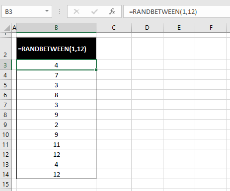
Evidently, there are many repetitions of values. One way around this can be to substantially expand the range supplied to the function to decrease the chances of duplicates. Let’s try 1 to 1000 and see how the RANDBETWEEN function responds to that:
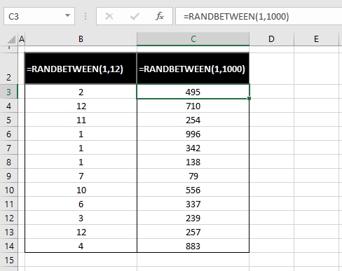
RANDBETWEEN is also a volatile function. For the values to stay, paste the values onto themselves.
By the look of it, we may not have repeated values. A surefire check can be performed using the Remove Duplicates feature. Select the values you want to check for duplications, paste the values onto themselves and then go to the Data tab > Data Tools group > Remove Duplicates button:
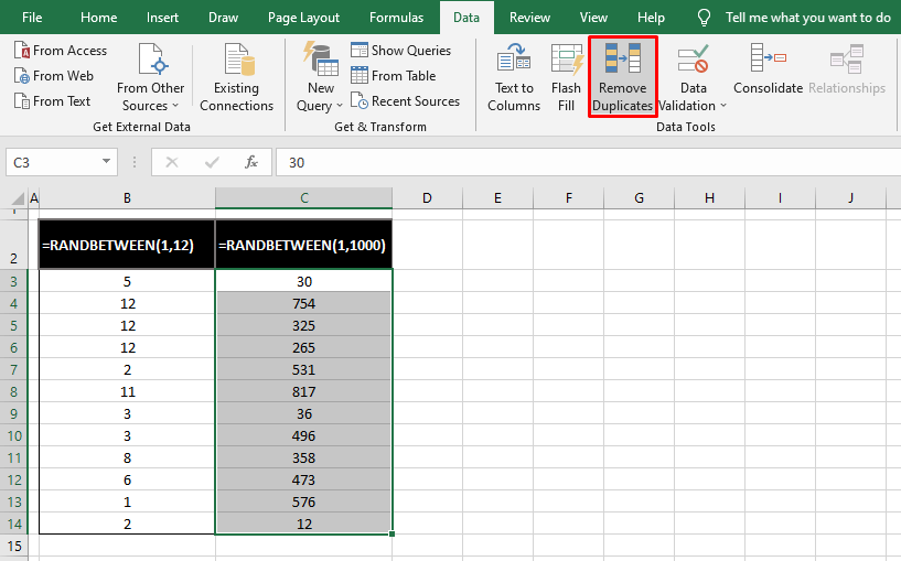
Select the Continue with the current selection radio button in the Remove Duplicates Warning dialog window.
Then select the Remove Duplicates button.
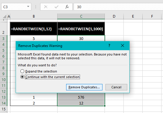
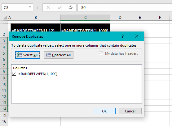
Click on the OK command button in the next window:
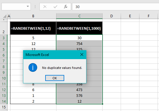
If there are no duplicates, you will see a small window confirming so:
If there are duplicates, you can have them removed using this feature and keep the values left over.
Method #3 – Using RANDARRAY Function
The RANDARRAY function returns an array of random numbers. The range between which the random numbers are to be returned, the number of random generations, decimals, or whole numbers, all can be defined.
However, like RANDBETWEEN, it returns duplicate values so all the tips of expanding the range or using RANDARRAY with other functions to avoid duplicates, apply here too.
Let’s see the simple application of the RANDARRAY function to generate random numbers:
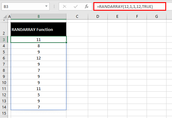
=RANDARRAY(12,1,1,12,TRUE)All the arguments are optional and if all of them are left out, RANDARRAY returns one random decimal between 0 and 1 (like the RANDBETWEEN function).
In our formula, the first 12 is the number of rows to be filled by the function followed by the number of columns, which we have specified as 1. The next two values (1,12) define the range for random number generations. TRUE returns integers and FALSE or omission of this argument returns decimals.
The results spill to the specified range so you don’t need to copy the formula down. Here’s what our formula looks like on the sheet:
Method #4 – Using RAND & RANK Functions
The RANK function returns the rank of a certain number in a list of numbers. This can make the RAND function more useful for random number generation. The RAND function will return random decimals and the rank function will rank the numbers according to their values. This will result in a set of random numbers without duplications.
Here’s what to do to generate a list of random numbers with the RAND and RANK functions:
- Apply the RAND function as follows and copy the formula down to as many cells of random numbers as required.
=RAND()The RAND function is used plainly to return a list or random decimals between the numbers 0 and 1. For our example, we require 12 random numbers so we have filled the formula down to eleven more cells:
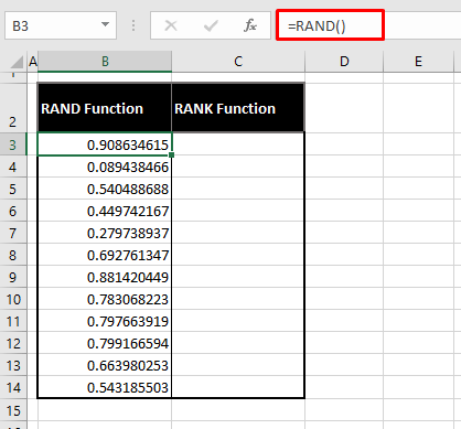
- In a new column, enter the following formula:
=RANK(B3,$B$3:$B$14)The RANK function will define the rank of a decimal generated by the RAND function. RANK is required to return the rank of cell B3 in the range B3:B14. The range is locked by dollar signs to avoid the repetition of numbers. The numbers will be repeated because as the formula moves down, the range will also move down, leaving out the decimals from the top and defining the rank of the specified cell in a new range every time.
To lock the cells into absolute references, press the F4 key with the blinking text cursor positioned after the cell reference in the formula bar.
The third optional argument of the RANK function is the order by which the function is supposed to rank the numbers. If left out, the function by default ranks the numbers by descending values; the first being the largest number.
- Drag the formula down to C14 to get all the numbers ranked and to get a list of 12 numbers at random.
You can see below that the number ranked as 1 is the largest number in the range B3:B14 and the one ranked as 12 is the smallest:
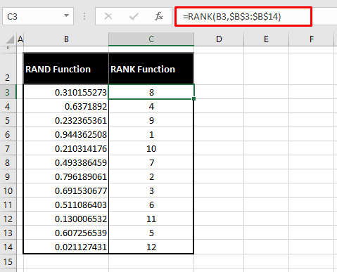
At this point, the results of the RAND function are volatile, making the results of the RANK function volatile too. It’s a good idea to leave it volatile until this point so you can recalculate the numbers if you don’t like the order.
- Once you have the results of the RANK function, copy the C column and paste the values on themselves to avoid the values recalculating and to avoid reference errors when column B is deleted.
- Delete the column with the RAND function.
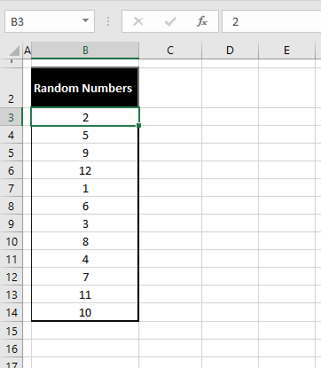
Method #5 – Using RAND, LARGE & MATCH Functions
The LARGE function returns the nth largest value in a dataset. The MATCH function is a lookup function that returns the position of a lookup value in an array. The RAND, LARGE, and MATCH can be used to return a random set of numbers, similar to using the RAND and RANK functions.
The RAND function will be used to generate random decimals that the LARGE function will arrange in descending order. Then the MATCH function will be used to look up each value from the LARGE function to result in its position in the list of decimals from the RAND function.
This is how to use the RAND, LARGE, and MATCH functions to generate a random set of numbers without repetitions:
=RAND()- The first step again is to use the RAND function with no arguments for returning random decimals:
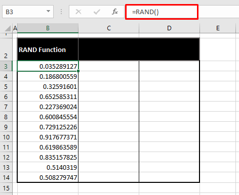
- Enter the following formula with the LARGE function:
=LARGE($B$3:$B$14,ROW(A1))The LARGE function takes the values in the range B3:B14 generated from the RAND function. This range is an absolute reference in the formula so that no value is missed out as the formula is copied down.
The second argument of the function is N in terms of defining the Nth value. Since we want this value to change in sequence as the formula is copied down, we have mentioned the ROW function with cell A1. This could be any column (e.g. B1, C1, or D1) as the ROW function will only deal with the row number. We have started with 1 so that the formula can change to row 2,3,4, so on as the formula will be filled down.
For the first instance, the ROW function returns the number 1 with A1 as the argument. That means the LARGE function has to find the 1st largest value in the range B3:B14.
In the second instance, the argument of the ROW function will change from A1 to A2. LARGE is to find the 2nd largest value in B3:14. That’s how this formula will work all the way down to the 12 values and it arranges all the values from the RAND function in descending order.
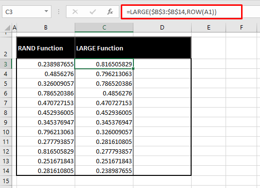
- Next, use the following formula in a new column:
=MATCH(C3,$B$3:$B$14,0)Now the MATCH function will look up the position of the value of cell C3 in the mentioned array B3:B14. The zero at the end is used by the MATCH function to find an exact match. As the MATCH function keeps finding the position of each value in B3:B14, it will keep returning the positions, supplying us with a list of random numbers.
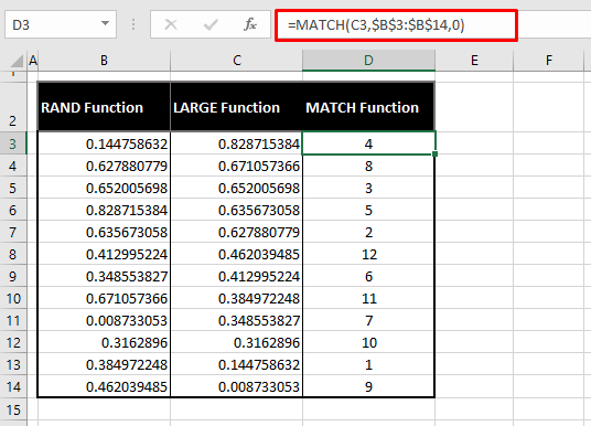
- Copy-paste the values of the MATCH functions onto themselves to prevent reference errors when the other two columns are deleted.
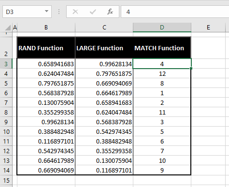
- Delete the columns with the RAND and LARGE functions.
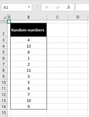
Method #6 – Using VBA
If you’d rather be interested in the works of coding, many codes can generate random numbers. Decimals or integers, pop-ups or lists, single or multiple values. You only need the relevant code. That code will work through VBA to generate random numbers.
As with all random generations, the question is – Will there be any repeat values? Yes and no; we have two codes for you here, one of them returns duplicates and one doesn’t. These codes can be edited to your requirements with minimum and maximum values and the number of random generations.
From all the types of VBA random number generations, we will show you how to get a list of 20 integers on your worksheet. Without further ado, let’s get into the steps of generating random numbers using VBA:
- Go to the Developer tab > Code group > Visual Basic button to open the VB editor. If you don’t have the Developer tab showing on the ribbon, you can press the Alt + F11 keys. This is the VB editor:
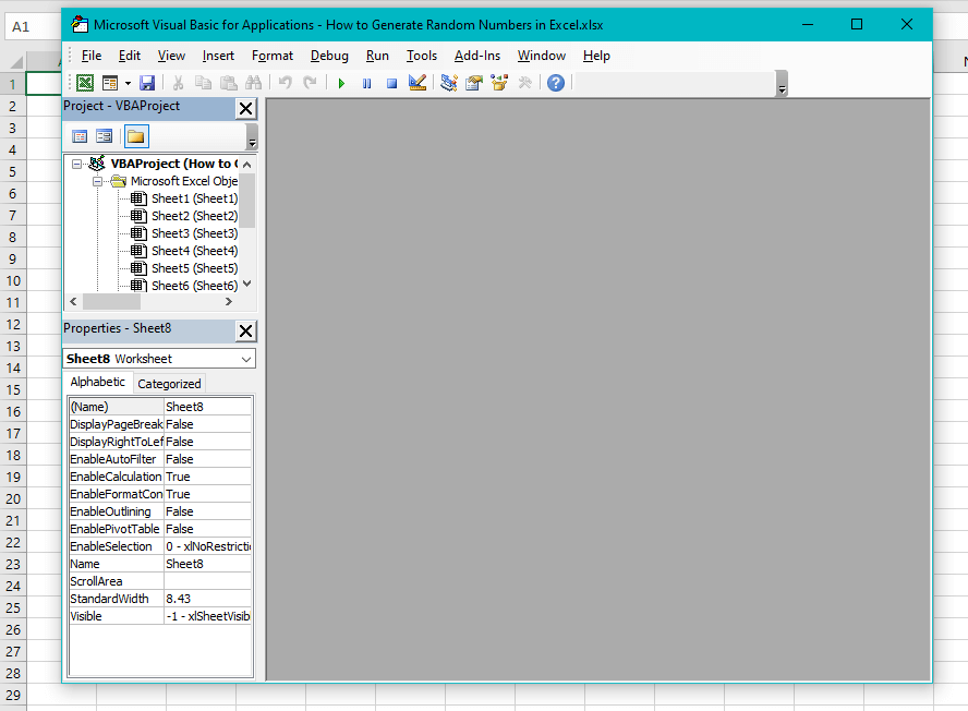
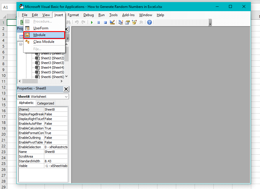
- Select the Module option from the Insert tab’s menu. This will open a Module window for feeding the code.
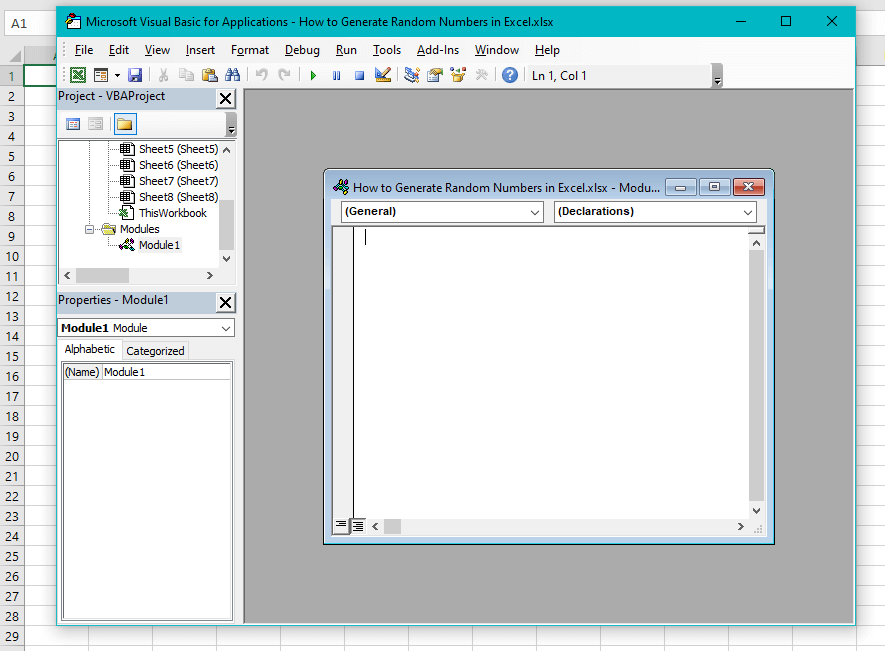
Here’s the Module window:
With Duplicates
If duplicate values are not a problem, go with this code:
- Copy-paste the following code into the Module window:
Public Function RandomNumbers(Num1 As Long, Num2 As Long, Optional Decimals As Integer)
Application.Volatile
Randomize
If IsMissing(Decimals) Or Decimals = 0 Then
 RandomNumbers = Int((Num2 + 1 - Num1) * Rnd + Num1)
Else
 RandomNumbers = Round((Num2 - Num1) * Rnd + Num1, Decimals)
End If
End Function
The function sets the values to return as whole numbers:
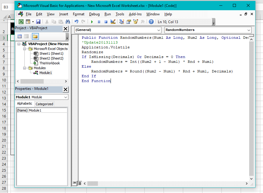
- Close the VB. Now you should be back to your worksheet.
- Enter this formula in the cell where you want the first random number:
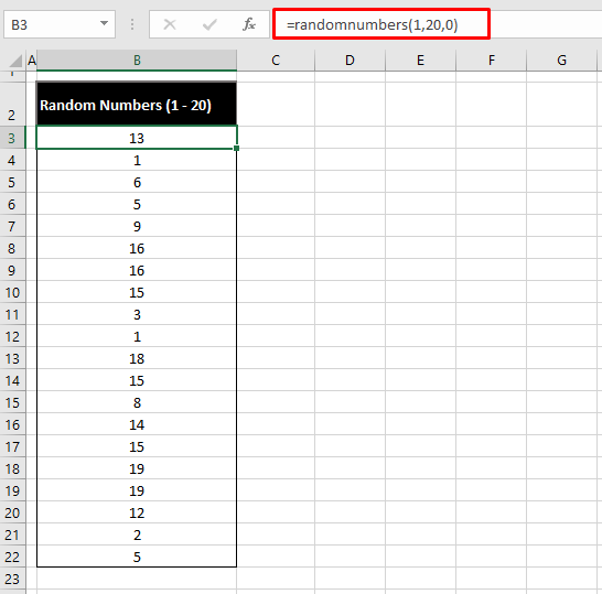
=RandomNumbers(1,20,0)This formula connects with the code fed through the VB editor. 1 and 20 are the bottom and top values between which you want the random number of generations. 0 is the number of decimal places you want in the generated values.
Here are the 20 random numbers generated using the VBA code and the formula mentioned above:
Without Duplicates
For unique random numbers, enter this code instead:
- In the Module window in the VB editor, copy and paste the code below:
Sub RandomNumbers()
Const Min As Long = 1
Const Max As Long = 20
Const HowMany As Long = 20
Const StartRow As Long = 3
Const Col As String = "B"

Dim LastRow As Long
Dim Ws As Worksheet
Dim i As Long, j As Long, Temp As Long, Number As Long
Dim Arr

If Max = 0 Then
 MsgBox "Maximum number can not be 0"
 Exit Sub
End If

If HowMany = 0 Then
 MsgBox "Number of required Randoms can not be 0"
 Exit Sub
End If

If Min > Max Then
 MsgBox "Minimum is more than Maximum"
 Exit Sub
End If

If Max - Min + 1 < HowMany Then
 MsgBox "Number of Randoms required should not be more than Max - Min + 1"
 Exit Sub
End If

Set Ws = Worksheets("Sheet1")
Application.ScreenUpdating = False
Number = Max - Min + 1
ReDim Arr(1 To Number, 1 To 1)
For i = Min To Max
 Arr(i - Min + 1, 1) = i
Next i
Randomize

For i = 1 To Number
 j = Int((Number - i + 1) * Rnd) + i
 Temp = Arr(i, 1)
 Arr(i, 1) = Arr(j, 1)
 Arr(j, 1) = Temp
Next i

Ws.Range(Col & StartRow & ":" & Col & StartRow + HowMany - 1) = Arr
Application.ScreenUpdating = True
End Sub
Don’t be intimidated by the length of the code, it works!
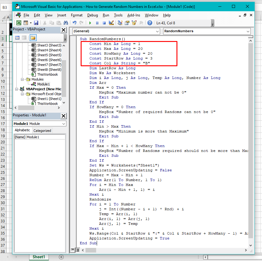
This is the part of the code you can edit as per requirement:
| Statement | Description |
|---|---|
| Const Min As Long = 1 | Minimum value |
| Const Max As Long = 20 | Maximum value |
| Const HowMany As Long = 20 | Number of random generations |
| Const StartRow As Long = 3 | Starting row number |
| Const Col As String = "B" | Starting column |
- Press the F5 key to run the code. The numbers should appear on the worksheet in the location specified in the code.
- Exit the VB
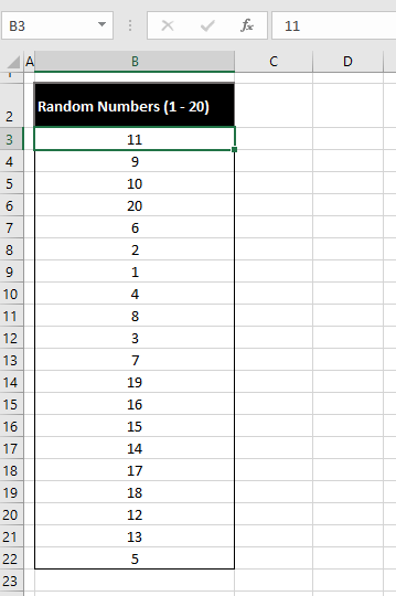
These are the 20 randomly generated numbers without duplicates, using the monster VBA code from above:
Now let’s generate an end to this all. We hope you find our methods easy to follow and easily customizable. Next time you’re wondering how to generate random numbers, you don’t have to download a random number generator; you can come back to our non-random tutorial on random numbers. Work your fingers on some random magic while we work ours to ready your spellbook!


