How to Get All Worksheet Names in Excel (2 Easy Ways)

You have made a decision. You are, Excel-ly, not walking the manual route unless you must. Whether the file contains a single worksheet or a single hundred, putting together a list of all the worksheet names is not a situation demanding that you take the manual route so here we are. Welcome to Exceltrick's guide on getting all worksheet names in Excel so you can focus your skills and energy on other requirements.

Our tutorial comprises getting sheet names in Excel using a formula and a couple of VBA codes. Also, find out how to add hyperlinks to up your Excel game.

Let's get working!

Method #1 – Getting Sheet Names Using Formula

We'll be getting all our sheet names with a formula but the formula isn't being applied conventionally, straightaway in the target cell. We need a small background working to patch up our formula. A named function will be created so that the name can be used in the formula on the worksheet to return all the sheet names in the workbook.

The function will be named using the Name Manager and the detailed steps ahead will give you the rest of the story on how to get all the worksheet names in Excel:

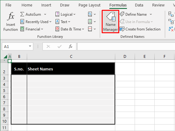
• Go to the Formulas tab and click on the Name Manager in the Defined Names group to launch the Name Manager.
• Alternatively, you can open the Name Manager using the Ctrl + F3 keys.
• 
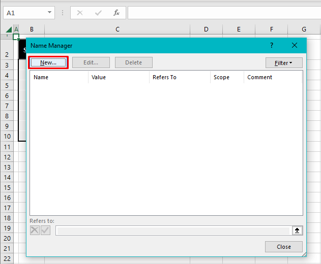
• Select the New button in the Name Manager.
• 
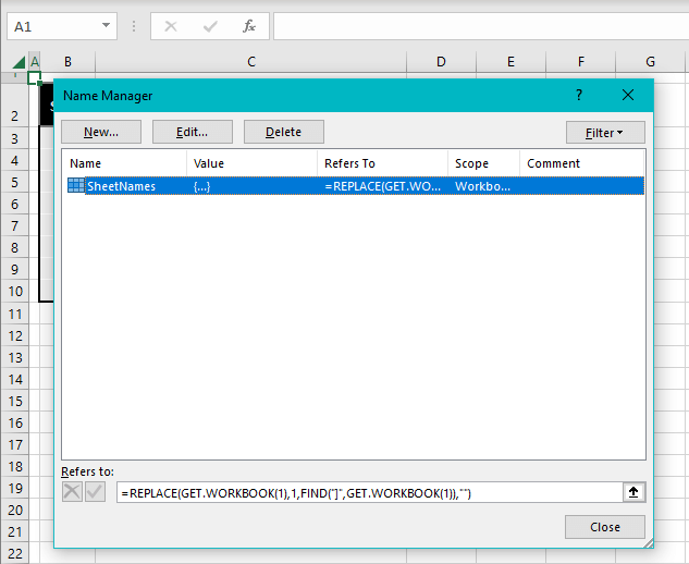
• Enter the details to create the named function.

Add a name of choice in the Name field as we have added SheetNames.

Keep Workbook as the Scope.

Copy and paste the following formula in the Refers to field:

In the formula, =GET.WORKBOOK(1) returns all the sheet names of a workbook prefixed with the workbook name and file extension enclosed in square brackets. E.g., if the workbook name was MyWorkbook, =GET.WORKBOOK(1) would return [MyWorkbook.xlsx]Sheet1 as the first sheet name.

The rest of the formula works to replace the file name with empty text using the REPLACE function so that we are left with just the sheet name. 1 in the second argument indicates the starting point of the replacement text. The endpoint for the replacement is given in the third argument through the FIND function. REPLACE is to replace the text starting from the first character of the workbook name (i.e. the opening square bracket) to where the FIND function finds the closing square bracket in the workbook name.

Replacing the text from the opening to the closing square bracket will eliminate the prefixed file name and leave just the sheet name as Sheet1.

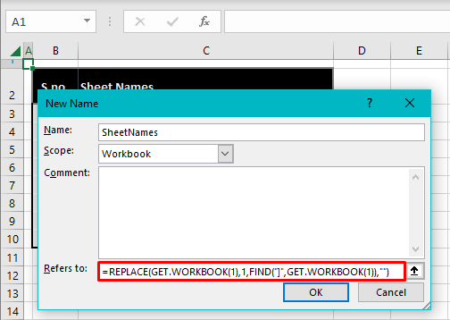
• After entering the formula, hit the OK command to create the named function.
• Now you will see the new named function in the Name Manager, ready to be used as a name in a worksheet formula.
• 
• Close the Name Manager.
• In a separate column, before the column intended for the sheet names, add serial numbering. This numbering represents the number of sheets in the workbook.
• Next, add the following formula to the target cell, where you want the sheet names to begin.

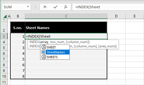
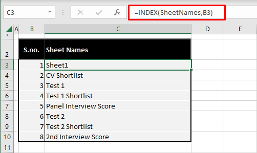
Use the named function in the INDEX formula to get all the sheet names, minus the prefix of the file name. When typing out the formula, the named function will appear in the Formula AutoComplete:

With the formula applied using the created name, we have all the names of the workbook's worksheets listed below:

Method #2 – Getting Worksheet Names Using VBA

Other functions can be used as names in formulas to create a list of the worksheet names and you can also employ VBA for the same job. Use a code in VBA that will itemize all the worksheet names from the workbook to the target location on the active worksheet. Read the steps given ahead to learn how to get sheet names in Excel using VBA:

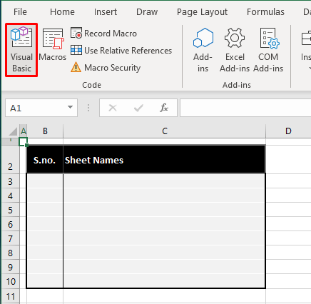
• Use the Visual Basic button in the Developer tab's Code group to access the Visual Basic You can directly use the Alt + F11 keys for the Visual Basic editor if the Developer tab is disabled on your Excel.
• 
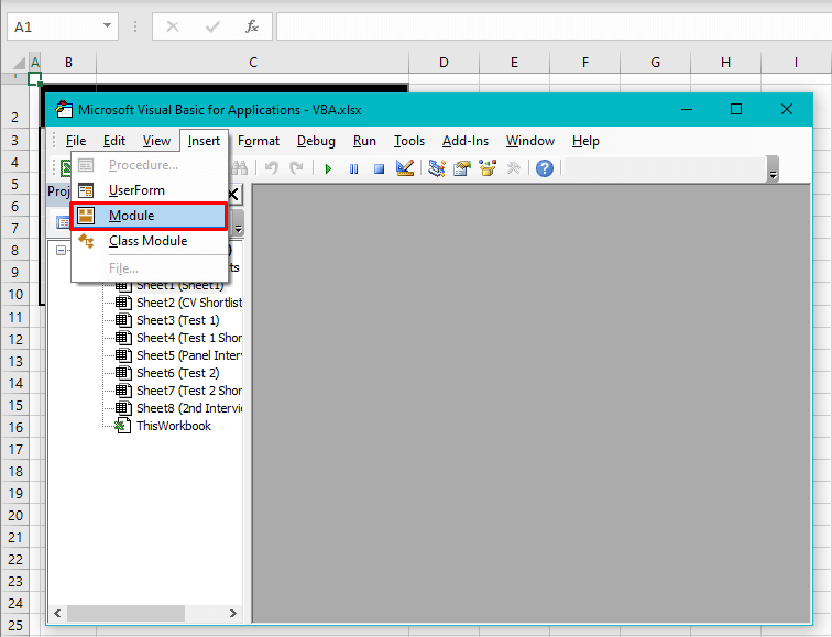
• With the Visual Basic editor now open, click on the Insert tab above the toolbar and select Module.
• 
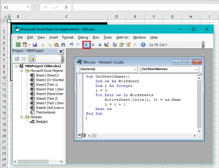
• In the Module window that has opened, copy and paste this code for getting the worksheet names:

• Sub GetSheetNames()
  Dim ws As Worksheet
  Dim i As Integer
  i = 3
  For Each ws In Worksheets
   ActiveSheet.Cells(i, 3) = ws.Name
   i = i + 1
  Next ws
  End Sub

  You can change the location of where you want the names listed on the worksheet. i = 3 in the 4th line of the code refers to the row number the sheet names will be enlisted from. Change 3 in the 6th row of the code from ActiveSheet.Cells(i, 3) to change the column number of the starting location for the list. We want our list to start from C3 (i.e. column 3 and row 3) so we've set both the row and column number as 3.The code will add all the sheet names in the provided cell location on the active worksheet.

• When done setting the code, use the Run button from the toolbar or the F5 key to run the code.
• In the background of the Visual Basic editor, the worksheet names will be enlisted as soon as you run the code.
• Close the Visual Basic

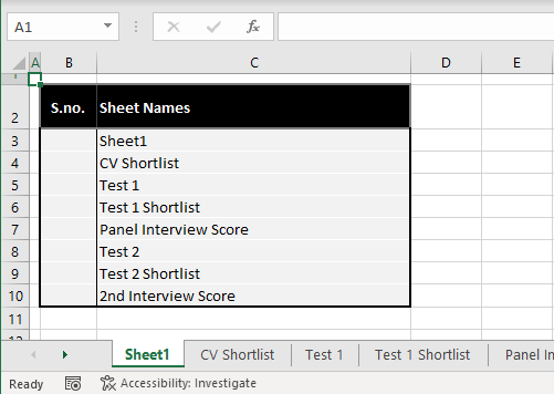
We got you the list. You add the serial numbers. If you must.

Creating Worksheet Hyperlinks

Aren't we fans of all things that are just a click away? Yes, we are and that is the promise that comes with hyperlinks. Instead of clicking through the worksheet tabs before you find what you're looking for, you can use a clickable link with all the worksheet names to land you on the chosen worksheet, courtesy of the HYPERLINK function. The HYPERLINK function creates a shortcut, opening a document on your computer or the internet.

Since hyperlinks are an added feature, we'll expand on our example workbook from above and create worksheet hyperlinks with the extracted worksheet names. Here's what you need to do after extracting the sheet names:

In a free column, add the following formula against the first worksheet name:

It might look like this formula is housing a lot but it's just two arguments: the link location and the hyperlink name. Therefore, "Go to Sheet" after the comma in the formula is the hyperlink name or the anchor text that will appear once we've applied the formula. Its appearance will be that of a regular hyperlink: the underlined name in blue font.

Now for the part in the formula that is before the comma; this is the link location, the point where the created link will take you. In our case, we need it to take us to the selected worksheet in the same workbook. The hash sign, exclamation mark, and double quotes are a way of adding the cell and sheet references as the location.

A pair of double quotes enclose the hash sign and also !B2 while single quotation marks enclose &C3&. The hash can be joined to the cell reference C3 but C3 needs to be separated and enclosed in single quotes when there are spaces in the worksheet name. The cell reference C3 is used since we have the sheet names listed in column C. C3 is wrapped in ampersands (&) to keep the cell reference relative so that as the formula is copied down, the next sheet name from C4 will be taken.

B2 is the cell on the destination sheet that the hyperlink will land us on. And that is how the formula is pieced together, folks. See the hyperlinks we've created using this formula:

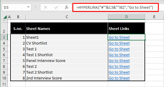
Create your worksheet hyperlinks and use them. You know you want to.

Bonus: Creating Dynamic Sheet Names List

With hyperlinks. That's right! In this section, you'll find an easy way of creating a dynamic list of all the worksheet names in the workbook. The new list will come with another perk, or two; the list will be created in hyperlinks, also hyperlinking back to the sheet with the list.

Since that can require some attention to detail, we'll just dump all the responsibility on a VBA code and get going. The following steps are on making a hyperlinked list of all the worksheet names in Excel:

Note: You can choose any sheet for housing the list but bear in mind that the name of the target sheet will be skipped from the list without any gaps; the name of the sheet before and after the target sheet will be listed one after the other. In our case example, we are using the first sheet (Sheet1) as the target sheet for the list.

• Set the target sheet for creating the sheet names list.
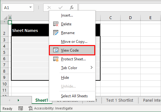
• Right-click the tab of the target sheet and select View Code from the menu.
• 
• You will be redirected to a Code window in the Visual Basic editor.
• Copy the code provided below and paste it into the Code

• Private Sub Worksheet_Activate()
  Dim xSheet As Worksheet
  Dim xRow As Integer
  Dim calcState As Long
  Dim scrUpdateState As Long
  Application.ScreenUpdating = False
  xRow = 2
  With Me
   .Columns(1).ClearContents
   .Cells(1, 1).Name = "Index"
  End With
  For Each xSheet In Application.Worksheets
   If xSheet.Name <> Me.Name Then
   xRow = xRow + 1
   With xSheet
   .Range("A1").Name = "Start_" & xSheet.Index
   .Hyperlinks.Add anchor:=.Range("A1"), Address:="", _
   SubAddress:="Index", TextToDisplay:="Back to Index"
   End With
   Me.Hyperlinks.Add anchor:=Me.Cells(xRow, 2), Address:="", _
   SubAddress:="Start_" & xSheet.Index, TextToDisplay:=xSheet.Name
   End If
  Next
  Application.ScreenUpdating = True
  End Sub

  Like before, you can change the cell location that the list will start from. 7th line of the code, change 2 according to the row number you want as n-1. E.g. we're aiming for the list to begin from row 3 so we have entered 2 (which comes from 3-1) here.
  The column number will be changed from the code's 4th last row. Change 2 as per the column number of choice. A1 in the 16th line signifies the cell of the sheet that you will jump to when you click that sheet's hyperlink from the list.
  "Back to Index" in the 18th line will be the anchor text of the hyperlink leading back to the sheet with the list. Change this text if you so wish (e.g. Back to List, Go to List, Go Back). A1 in the 17th row is the destination cell of the Back to Index hyperlink. When you use the link to get back to the sheet with the list, you will arrive at cell A1 i.e., the start of the worksheet.
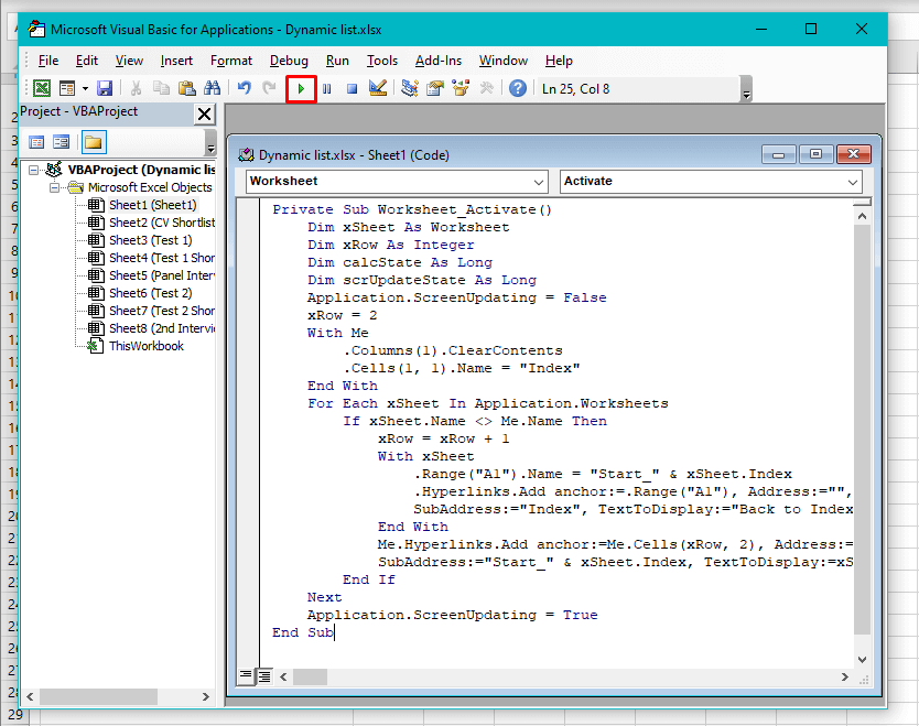
  This is how the code will appear in VBA:

• Run the code using the F5 key or the Run

And that's the hyperlinked list of all the workbook's worksheet names.

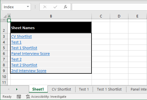
Clicking on the last link, we are directed to the selected sheet with the return link in cell A1:

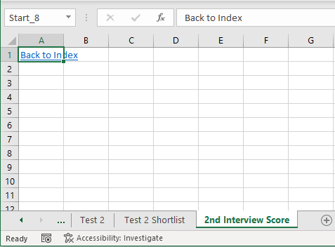
Let's test the main purpose of this exercise, the list's dynamic quality. We're adding a new sheet to see if the list responds.

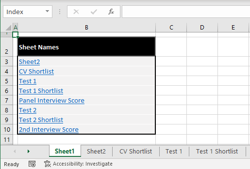
It does! The return link will not be instantly created in the new sheet but it will, once you visit the main sheet and let the list update automatically. The list will respond to additions, deletions, and position changes of the worksheets.

So that was how to get all the worksheet names listed in Excel. Now you know 2 easy ways to do that, involving built-in and segregated hyperlinks. We'll catch you with another Excel situation rounding the corner!