Highlight Entire Row in Excel With Conditional Formatting

Learn how to highlight rows in Excel with Conditional Formatting in this tutorial. We have detailed methods on highlighting rows according to text or numbers, multiple conditions, and blank cells all using Conditional Formatting. Also learn a really cool trick to highlight rows based on the value entered in a separate cell.

Conditional Formatting is an Excel feature that applies specified formatting to cells that meet the supplied criteria. Also, Conditional Formatting is dynamic; it adapts to added, deleted, and edited data. So everything you learn below will be applied to your data dynamically.

You often need values highlighted in datasets, some as a red flag and some as a green flag because they satisfy certain criteria. Since these values are the particulars of a product or person, it would help to have the full row highlighted so you don't have to eye the highlighted cell first and then see what product or person it is about. A little explanation on how this works before we get down to the methods.

Let's get highlighting!

Highlighting Entire Row Vs Highlighting a Cell

If you were to directly head to Highlight Cell Rules in Conditional Formatting, you would be highlighting individual cells. Let's show you an example and explain how highlighting the row instead of just the cell works. Take this dataset as an example:

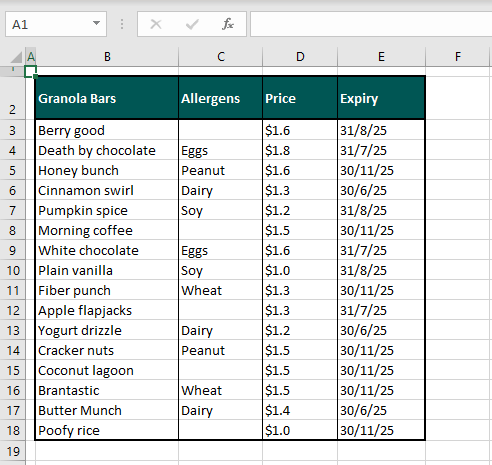
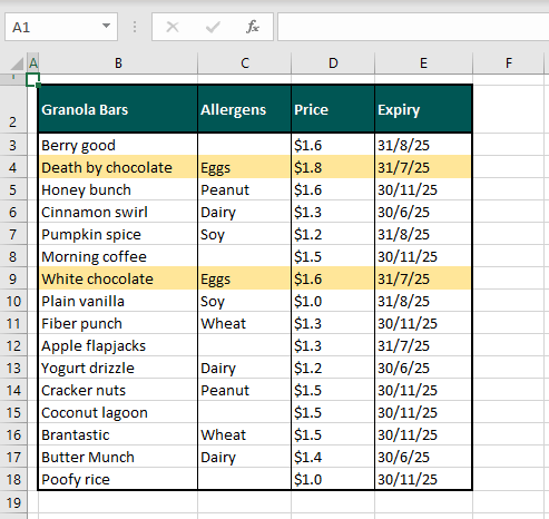
We have a list of granola bars and want to search for bars that contain eggs as an allergen. Instead of just highlighting the allergen in column C, we want the whole product highlighted which means we want to highlight the full row. Using Conditional Formatting, the rule we will set will be with this formula:

Only the column is locked in reference with a dollar sign, not the row. So the formula goes row by row checking the cells starting from row 3 as mentioned in the formula. While the formula searches row by row, it checks only column C as we have entered column C as an absolute reference. When the formula finds "Eggs" in column C, it highlights the whole row. It also helps to select the entire dataset instead of just the column to have the whole rows highlighted.

Highlight Rows Based on a Text Criterion

Setting a new rule in Excel's Conditional Formatting feature can help us highlight rows based on a text criterion. You may have a dense dataset of products and you need to find and highlight a product based on its name or some other textual quality. That is all too easy with Conditional Formatting.

Using our example, we want to find the granola bars containing the allergen eggs. We will use Conditional Formatting with a new rule to find the text "Eggs" in column C and highlight the rows. These are the steps to highlight rows based on a text criterion:

• Select the whole dataset, except the headers.

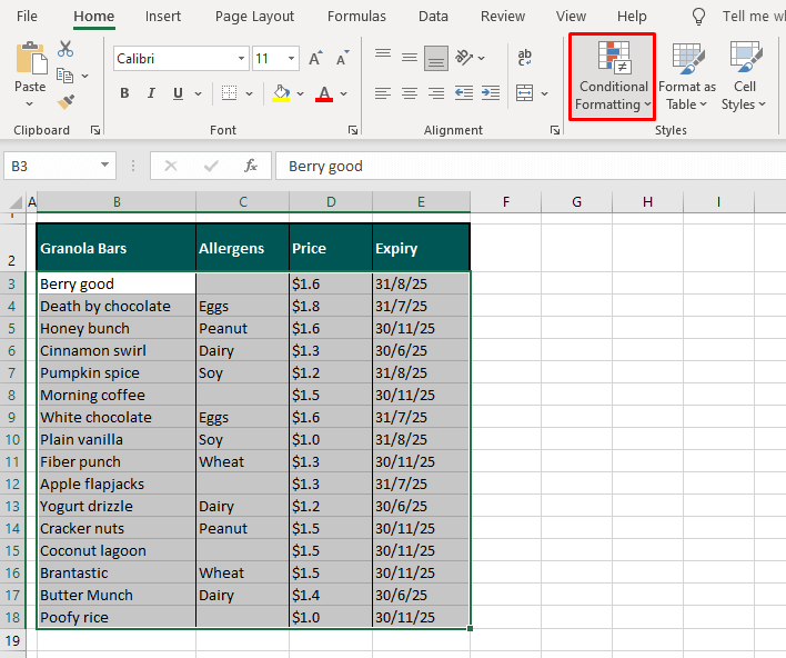
• In the Home tab's Styles group, select the Conditional Formatting button to open its menu.
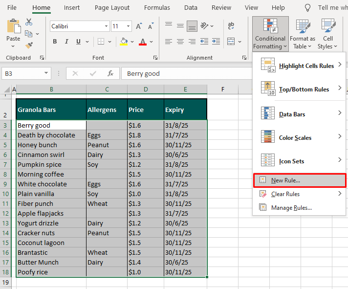
• Select New Rule… from the menu to open the New Formatting Rule window.

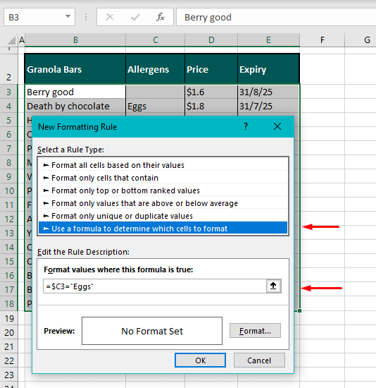
• Select the last rule type "Use a formula to determine which cells to format".
• In the field provided for the formula, enter the formula:

C3 is the first cell from the column containing the word you are searching for, preceded by a dollar sign $.

"Eggs" is the word you are looking for, enclosed in double-quotes.

Note that the dollar sign is used before column C to lock the search for the word only in column C.

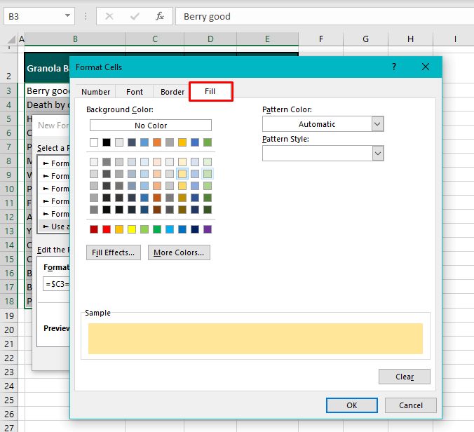
• Click on the Format… button to open the Format Cells window and then go to the Fill tab to select a color for highlighting the rows.

• Click the OK button on both windows to close them. The rows with the word "Eggs" in column C will be highlighted:

Highlight Rows Based on a Number Criterion

Using the same steps and concept as above, we can easily highlight rows based on a number criterion. Pretty much everything is the same as done earlier with a change in the formula and of course, a change in the column.

You could be looking to highlight clothing of a certain size or price, or quantities that need restocking. Extending our case example, we are aiming to highlight granola bars close to their expiry. We will show you the steps for this since formulating around a date is different than doing it for any regular number (we have a small formula example at the end of this section for simple numbers).

Below are the steps for highlighting rows based on a number criterion:

• Select all the cells in the dataset. Leave the headers out.
• Go to the Home tab > Styles group > Conditional Formatting button > New Rules… option. This leads to the New Formatting Rule window.
• In the Select a Rule Type: section, select Use a formula to determine which cells to format.
• In the Format values where this formula is true: field, enter the formula:

E3 is the first cell from the column where the date is to be searched, a dollar sign to lock the column.

The date is entered in the format (yyyy,m,d) as required by the DATE function.

*See note below on formulas for other numbers.

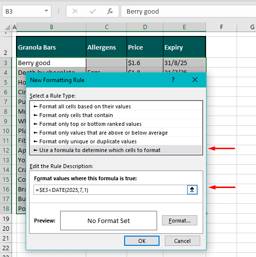
• Now set the color fill for highlighting the rows by clicking on the Format…
• This redirects us to the Format Cells window.
• Go to the Fill tab and choose the color for highlighting.
• Click on the OK button on the Format Cells window and then on the New Formatting Rule

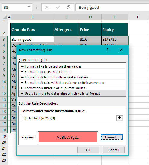
The rows with dates before 1-7-2025 in column E will be highlighted in the chosen color:

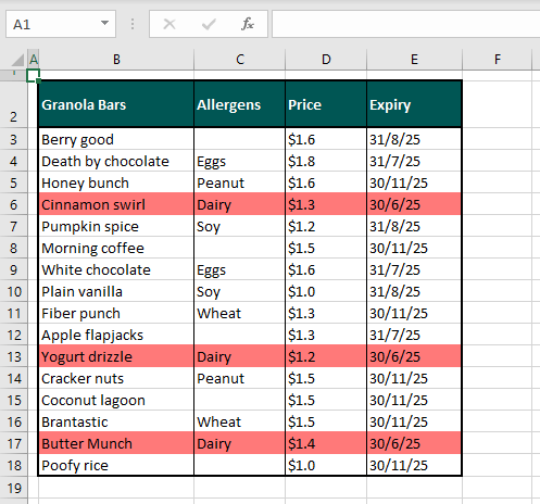
Note: Our example was based on highlighting rows falling before a certain date. If you are forming a rule based on other numeric figures such as price, quantities, etc., the formula would be quite simple. E.g. for finding granola bar prices above $1.6 in column D, the formula would be:

Highlight Rows in Different Colors Based on Multiple Conditions

With Conditional Formatting, we will show you how to highlight rows in different colors based on multiple conditions by adding 2 rules using the Conditional Formatting Rules Manager. Each rule will have its own color and criterion.

The first criterion we will add is to search column D for values greater than 1.6. The rows containing these values will be highlighted in blue. The second rule is to highlight the rows with values greater than 1.8 in green. Now let's see the steps for highlighting rows in different colors based on multiple conditions:

• Select the range including the dataset, excluding the headers.
• In the Home tab's Style group, select Conditional Formatting and then select the Manage Rules… options to access the Conditional Formatting Rules Manager.

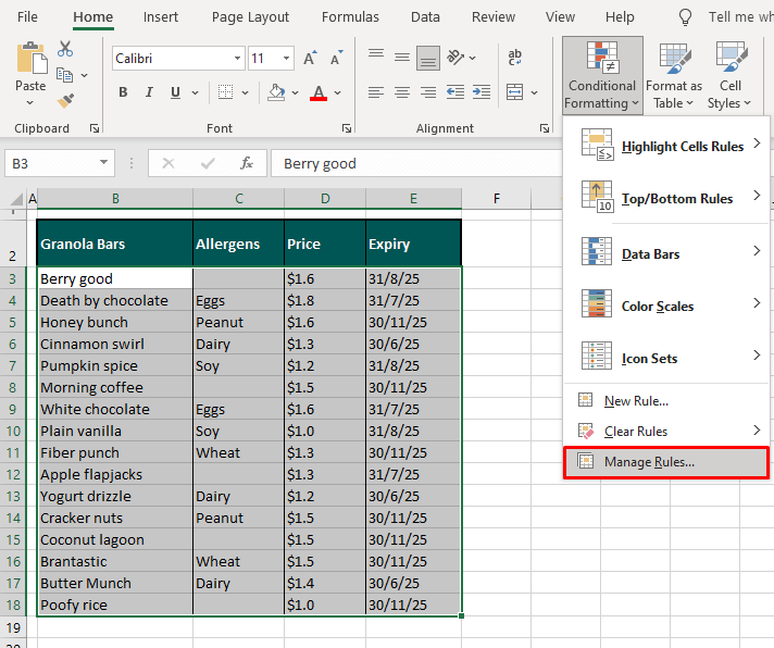
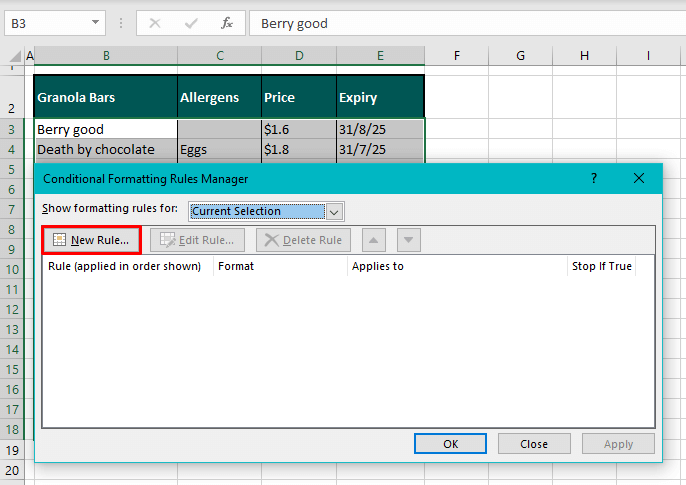
• In the Manager, select the New Rule… This will lead to the New Formatting Rule window.

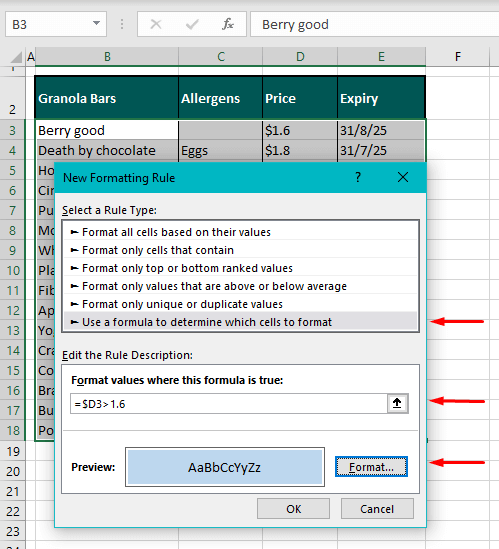
• These are the 3 things you need to do in the New Formatting Rule window:
• Select the last option in the Select a Rule Type. Enter your formula in the provided field. Here's the one we entered:

• We are using this formula to find the values greater than 1.6 in column D, starting from the first row in the dataset which is row 3.
• Set the color for highlighting the rows that this formula applies to by clicking on the Format button then selecting the color in the Fill

• Click on the OK command button when done. You will be redirected back to the Conditional Formatting Rules Manager.
• Select the New Rule… button again to add the second rule.

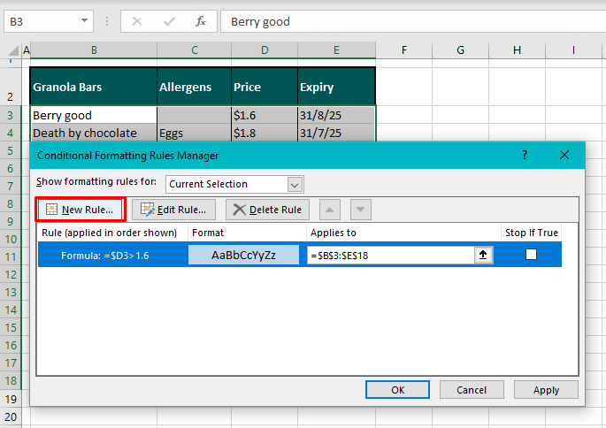
• Follow the same three steps as with the first rule. Choose the last option from Select a Rule Type.
• Add your second formula. This is what we added:

• Now we want to highlight the rows with values greater than 1.3 in column D. The first point of search is cell D3.
• Select the Format button and then the Fill tab to pick the color for highlighting the rows for the second rule.

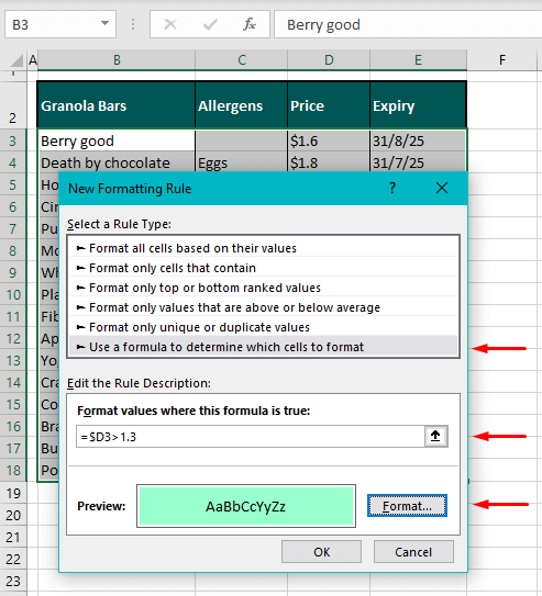
• Click on OK. Now you will be back to the Rules Manager with both the rules added.

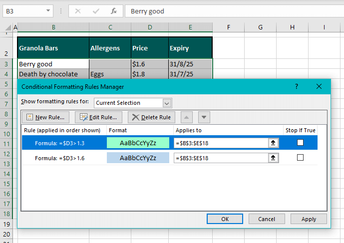
• Use the arrow buttons to rearrange the order of the rules. Explanation below*

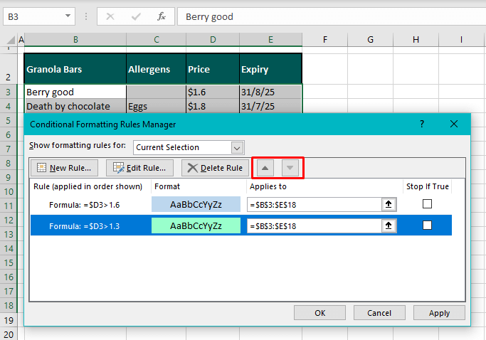
• Select the OK command button.

The rows relevant to the two rules will be highlighted in the respective colors:

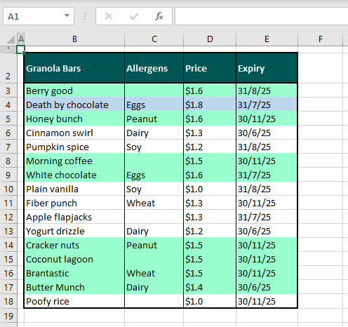
Note: The rule at the top gets priority and is applied before the second rule. For our case, we needed to have the first rule at the top. Had we left =$D3>1.3 at the top, all the values fulfilling the other rule =$D3>1.6 would also be greater than 1.3. That way, no row would be highlighted in blue since they have already fulfilled the criteria for the first rule.

Therefore, the rule at the top needs to be =$D3>1.6 so that the values greater than 1.6 are highlighted first and then the rest are left to be highlighted if they are greater than 1.3.

Highlight Rows Where any Cell is Blank

You may have heard of highlighting blank cells with Conditional Formatting but now we'll show you how to highlight the whole row if any one cell in that row is blank, from any column. Not different from what we've seen in the methods above; we create a new rule and use a formula and color for highlighting the rows with blank cells. These are the steps to do this:

• Leaving out the headers, select the dataset.
• Go to the Home tab > Styles group > Conditional Formatting button > New Rule…

• In the New Formatting Rule window make these changes:
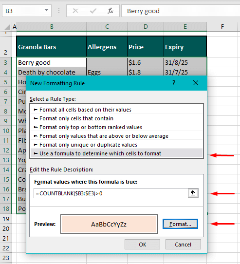
• Select Use a formula to determine which cells to format from the Select a Rule Type:
• Add the formula:

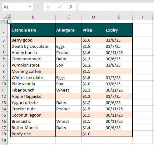
The COUNTBLANK function counts the number of empty cells in the range. The range included is all the columns of the dataset with the first row of the dataset. The COUNTBLANK function will count the number of blank cells in a row. If the result is greater than zero, that row will be highlighted.

• Select the color for highlighting the rows with blank cells using the Format

• Then click on OK.

The row containing a blank cell in any column will be highlighted:

Highlight Rows Based on the Value Entered in a Separate Cell

Jumping back to our first method, where we wanted to highlight the granola bars containing eggs, these were the results:

Now if you wanted to wipe out these results and highlight the rows with a dairy allergen, you would edit the formula and swap "Eggs" for "Dairy", right? How about you enter whichever allergen you want in a separate cell and it magically highlights the relevant rows?

The quick cap on that is to highlight a separate cell in the color being used for highlighting, yellow in our case. Label it for ease. Then edit the Conditional Formatting Rule from the Manager and include the separate cell in the formula instead of the value "Eggs". Then enter any allergen from column C and the rows containing the allergen will be highlighted!

Now here are the detailed steps to highlight rows based on the value entered in a separate cell:

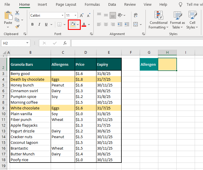
• Use the Fill Color button to highlight a separate cell in the same color being used in the dataset.
• Also label the separate cell as we have labeled it as Allergen below:

• To open the Conditional Formatting Rules Manager, go to the Home tab > Styles group > Conditional Formatting menu > Manage Rules…

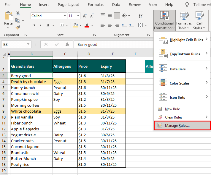
• Select the rule and click on the Edit Rule…

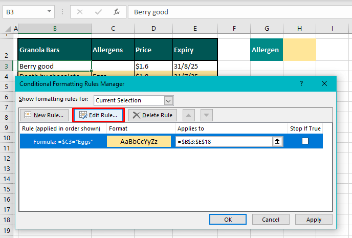
You will see an Edit Formatting Rule window with the current formula.

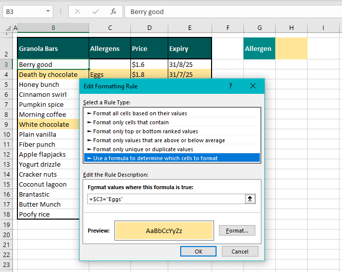
• Edit the formula: remove the value "Eggs" and replace it with the cell reference of the separate cell by clicking on it.
• The marching-ants line will appear when you click on the cell.

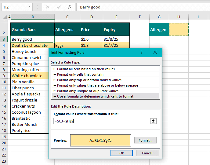
• Click on the OK button on both windows. Now enter a different allergen in the cell H2 and find its row highlighted:

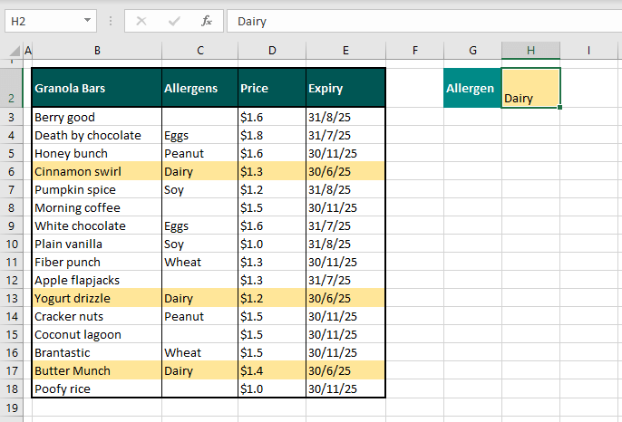
The color fill of the separated cell doesn't have an impact on the highlighting in the dataset but it's used more like a key code to show what the rows with the supplied value will be highlighted in.

And that's how we use Conditional Formatting to highlight not just cells but entire rows in Excel based on different conditions. You just need to know the formula you are working with and you'll be good. See you with more formulas and methods that you can work well with!