Ignore Blank Cells in Conditional Formatting (3 Easy Ways)

Conditional Formatting is the quickest and easiest way to add visual impact to any dataset but a Conditional Formatting Rule can be prone to its simplicity and might not be doing what you want it to do.

Our problem at hand, for now, is Conditional Formatting also highlighting blank cells when we would rather have them un-highlighted (and no one should be in the mood to do that manually. That's just wrong). But what's right is that there are two very simple solutions to this problem.

See this problem face to face:

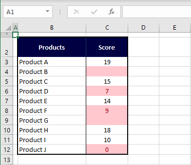
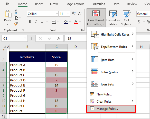
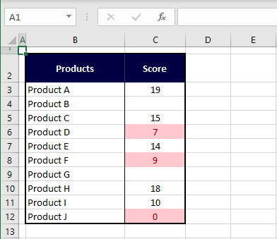
We're taking an example of quality scoring (out of 20) of various products. The ones left blank are the scores we are yet to receive. To highlight which products had scored less than 10 exclusively, we applied a "less than 10" Conditional Formatting rule which also highlighted blanks.

Why has that happened? Conditional Formatting sees blanks as a value being less than 10. The rule is posed to highlight all cells that have a value of less than 10 and while 0 is right to be considered less than 10, we don't want the blanks to be highlighted because technically, those products aren't even scored yet. Hence, it would be nice not to have our attention flitting to blanks unnecessarily.

Blank cells can be ignored in a Conditional Formatting rule with the addition of another rule that will disregard blanks. The rule can use the preset option of formatting blanks or we can use a formula with the ISBLANK function, either works just as well. You will also need to bump up the rule with the preference of the Stop If True option applied. Find out more about that later.

Also note that you are to use either of the 2 methods for ignoring blank cells in this tutorial if you want the cells with the number 0 to be highlighted. We will also talk later about a couple of fixes if you also want to avoid highlighting the 0-value cells.

This is probably not a good lead anywhere else in life but…

Let's get ignoring!

Recommended Reading: Conditional Formatting In Excel

Method #1 – Using Format Only Rule

The position we're sitting at right now is the one shown above; with the "less than 10" rule applied which has also highlighted the blank cells. We'll carry that forward as our case example and see what we can do to fix the highlighting of blank cells.

Our first method makes use of the Format only cells that contain rule in Excel's Conditional Formatting feature. We can set this rule to format or deformat only blank cells with the Stop If True option. With this option selected for a Rule, the other Rules will be "stopped" if a condition in this Rule is met.

Conceptually with us trying to ignore blank cells, if Stop If True is activated for the Rule we will create to deformat blank cells, the other Less Than Rule will be stopped if a cell is blank, to make way for the deformatting first. Further details and steps for this method are given below:

• Select the range with the Conditional Formatting rule (which will be C3:C12 in our case).
• Open the Conditional Formatting menu from the Home tab's Styles group and select Manage Rules.
• 
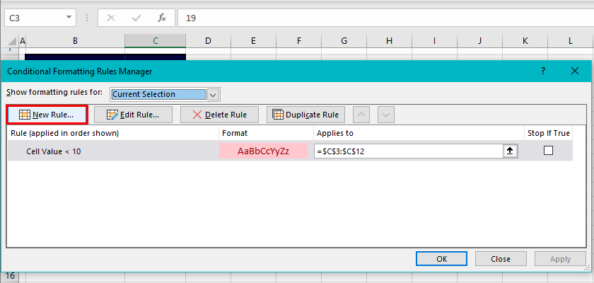
• This option opens the Conditional Formatting Rules Manager which shows the Conditional Formatting rules applied to the cells selected on the active worksheet.
• Click on the New Rule button on the top left of the Rules Manager.
• 
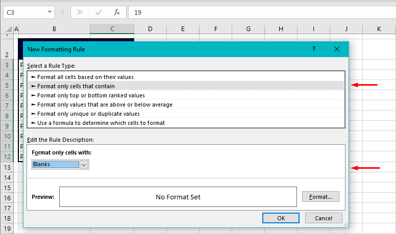
• In the New Formatting Rule dialog box, select the Format only cells that contain rule type.
• With this rule, 4 fields will now appear in the Rule Description area of the dialog box.
• Click on the arrow in the first field that reads Cell Value. Select Blanks from the drop-down list.
• 
• That's all you need to do here. Do not set any format for this rule.
• Click on the OK command in the dialog box.
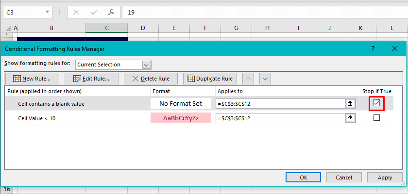
• You will be back to the Rules Manager where the newly created rule has been added. The rule will be ranked at the top which is where we need it to be. If not, select the new rule and use the upward arrow to place the rule at the top.
• Mark the Stop If True checkbox of the Cell contains a blank value
• This rule won't work if it isn't the first rule of the current cells selection even with Stop If True applied.
• 
• Now, Conditional Formatting will stop the application of the Cell Value < 10 rule if a cell is blank, skipping the highlighting of that cell.
• Select the OK button of the Rules Manager to close it and apply the new rule.

The rule regarding blank cells will be applied:

As can be noted, our problem of highlighted blank cells has been solved! The explanation is that when Conditional Formatting will pick up on a blank cell, it will inhibit the highlighting of the "less than 10" rule. When a cell isn't blank, Conditional Formatting will continue with the less than rule.

Method #2 – Using ISBLANK Function

The second method also involves creating a new rule but this time we're using a formula to stop blank cells from finding their way into the highlighting criteria with the ISBLANK function. The ISBLANK function returns TRUE if a cell is blank and FALSE if it isn't. Now let's test it in a Conditional Formatting rule to see if it does the job of ignoring blank cells.

We are again assuming that we applied the "less than 10" rule that has ended up with the blank cells highlighted. Follow the steps ahead to enter a new rule with the ISBLANK function to ignore blank cells in Conditional Formatting:

• Select the cells containing the formatting rule.
• Open the Conditional Formatting Rules Manager using the Manage Rules option in the Conditional Formatting
• 
• In the Rules Manager, select the New Rule
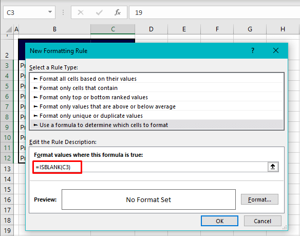
• In the New Formatting Rule dialog box, select the Use a formula to determine which cells to format rule type.

In the text box given in the Rule Description section, copy and paste this formula:

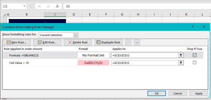
The ISBLANK function will deformat the highlighted blank cells. That is because we have not set a format for the blank cells in the new rule. This rule will work to change the blank cells to this unhighlighted format, consequently deformatting the blank cells.

Use the ISBLANK function with a relative cell reference and keep the rule free from added formatting.

• Return to the Rules Manager with the OK command in the dialog box.
• Check the Stop If True box of the rule with the ISBLANK formula.
• 
• Hit the Rule Manager's OK button

And we should have the blank cells clear of Conditional Formatting highlights:

Method #3 – Ignoring Cells with Zero and Blank Cells

That's all well and good but are you detecting a potential problem here? While we got Conditional Formatting to overlook blank cells, let's now suppose we don't require cells containing the number 0 to be highlighted either. That is because some users have entered unscored products as 0 and some have left them blank. There's an easy way to mend this so here's our suggestion.

You can set up a rule to deformat the cells that carry zero value, which will simultaneously work on blank cells too. The reason is that if it's zero itself that you want to leave out, blank cells, that Excel considers as zero will also be left out. To demonstrate the suggestion, let's snap back to our starting point of today; highlighted blank cells and 0 value cells with the "less than 10" rule applied to the range. Carry on with these steps:

• Select the cells on the sheet with the Conditional Formatting
• Open the Rules Manager from the Home tab > Styles group > Conditional Formatting icon > Manage Rules.
• 
• Use the New Rule button in the Rules Manager to form a new Conditional Formatting
• 
• From the Rule Type, choose Format only cells that contain.
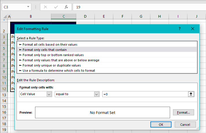
• In the Rule Description, select and enter these values in the provided fields: "Cell Value", "equal to", "=0"
• This rule will deformat cells with 0 as their value, along with blank cells.
• Hit the OK command when done.
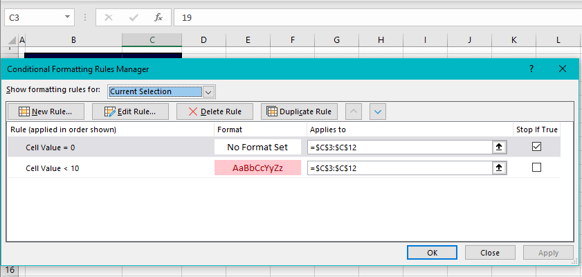
• Back to the Rules Manager, check the Stop If True box of the new rule.
• 
• Select the OK button to apply the rule.

You will find that the 0 value and blank cells have been ignored in the highlighting rule:

Tip: If applicable to your data, you can also edit the existing "less than 10" rule into highlighting values between 1 and 9 if you want to ignore blank and zero-value cells. This change will highlight numbers less than 10 and those greater than and equal to 1.

We're done with the ignoring part for today now that we're sure you've gotten a well enough idea of leaving out blank cells in Conditional Formatting. And even cells with 0 if required. While you're very busy with the ignoring part of things, we'll switch modes to enlightenment and hunt another Excel facet you won't be able to ignore!