How to Insert an Arrow in a Cell in Excel (6 Easy Ways)

The grand job of Excel is to be an analysis tool that gives a quick visual and graphic indication of data. Arrows also play a decent role in playing up to the quick visual part.

Pointing to denote the relation between data (datasets, objects such as lists, charts, and graphs) and showing increase and decrease in numerical values are the prime reasons for using an arrow in Excel.

By the end of this tutorial, you will learn a handful of ways of inserting an arrow in Excel that are copy-pasting and using the Symbol and Shapes options, Conditional Formatting, and special fonts.

There isn't one particular type of arrow that you're stuck with; there's a bunch of types you can choose from (line arrow, block arrow, pointer arrow, etc.) so why don't we start sampling some methods?

Let's get arrowing!

Method #1 – Copying & Pasting

In the first method, we are straight up serving the option to copy the arrow from here and paste it to your work. In this form, an arrow is a text value. Let's give you a little scenario and a small Excel trick to go with it; definitely a handy combo.

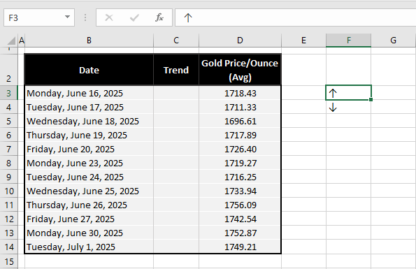
Suppose we have mapped the daily prices in dollars of an ounce of gold from 16^th June to the 1^st of July. To get an idea of the trend, we'd be eyeing a list of 6-digit numbers and what's the point of Excel if we have to strain so much?

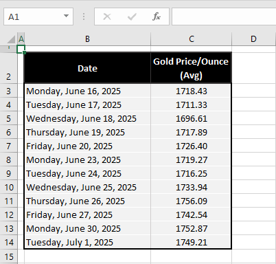
Here's our objective; we're going to add a new column to signify the trend of the gold prices with up and down arrows. Here are some arrows you might be interested in for your spreadsheet:

Now copy the up arrow and add it next to the increasing prices and the down arrow next to the decreasing prices. In the Excel world, that is actually a very caveman suggestion. We can make it much easier so, follow these couple of steps to insert arrows in Excel that are not so Stone Age:

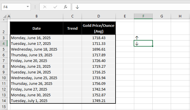
• Copy the up and down arrows of choice from above and paste them separately from your dataset on the worksheet:
• 
• Add the following formula to the trend column and copy it down so the arrows will be added for all the prices:

This is a simple formula with the IF function that goes: if the price (in cell D4) is greater than the earlier price (in D3), then insert the up arrow (in F3) otherwise, insert the down arrow from F4. F3 and F4 have been entered as absolute references so that the references do not shift as the formula is copied down.

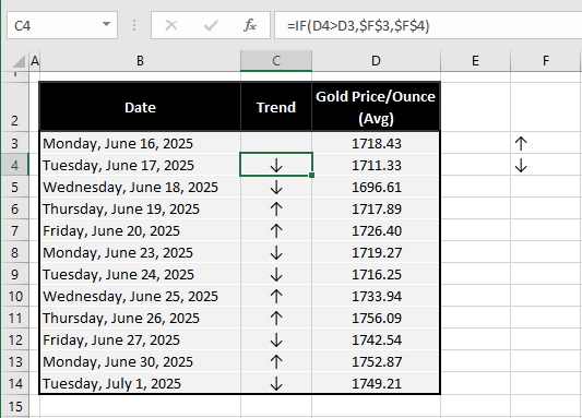
You can hide the off-dataset arrows in F3 and F4 by changing their font color to white. Being able to change the font color also hints that you can control the font style (including size, bold, and underline).

And that works to add the arrows in your data; no caveman in sight! Why this formula works is because the arrows in F3 and F4 are part of the cell's value. And the IF function is asking for the result to be the value of F3 otherwise that of F4.

Being a cell value, other characters can be added to the same cell as the arrow.

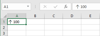
You can further make this outcome more visual by adding a Conditional Formatting layer to change the up arrows to red and down arrows to green. But if we must go the Conditional Formatting way, why not just go directly? You'll see how later.

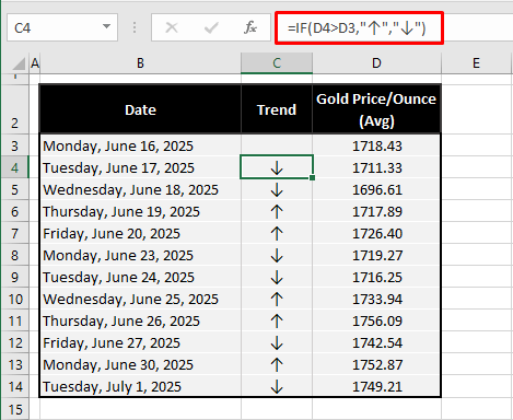
As a text value, arrows can be added directly in the formula like so:

Instead of using absolute references of the cells containing the arrows, we have copy-pasted the arrows straight into the formula. You can see that the results are identical and we've also eliminated the need to have the arrows in F3 and F4:

Method #2 – Using Symbol Option

For inserting arrows in Excel (or any symbol or character for that matter), nothing will give you a more diverse line-up than Symbol. Symbol is a tool in Excel that allows the user to add a character or symbol from a grand menu to the worksheet as a cell value.

Arrows aren't a very unusual character so you'll find many types in Symbol using plain and symbol fonts. See the steps ahead to insert arrows in Excel with the Symbol option:

• Select the cell where you want to add the arrow.
• We will be applying the IF function as shown in the example previously so the arrows are added away from the dataset.
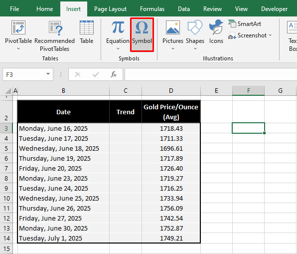
• In the Insert tab, select the Symbol icon from the Symbols
• 
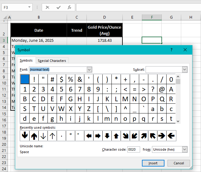
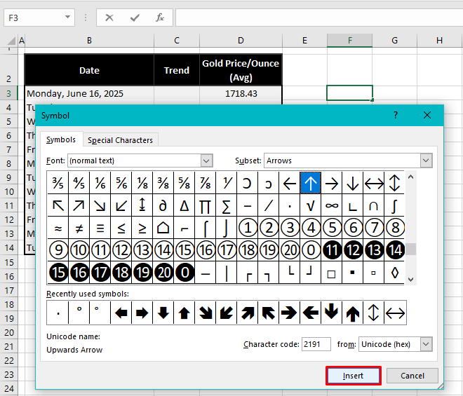
• This will launch the Symbol dialog box with a comprehensive spread of all types of symbols and characters imaginable:
• 
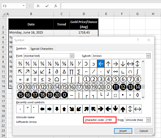
• Using the normal text in the Font bar given at the top, enter 2190 in the Character Code
• This is the code for a leftwards arrow preceding further arrow options including diagonal and double-pointed arrows.
• 
• Choose the arrow you want to add and then click on the Insert
• 
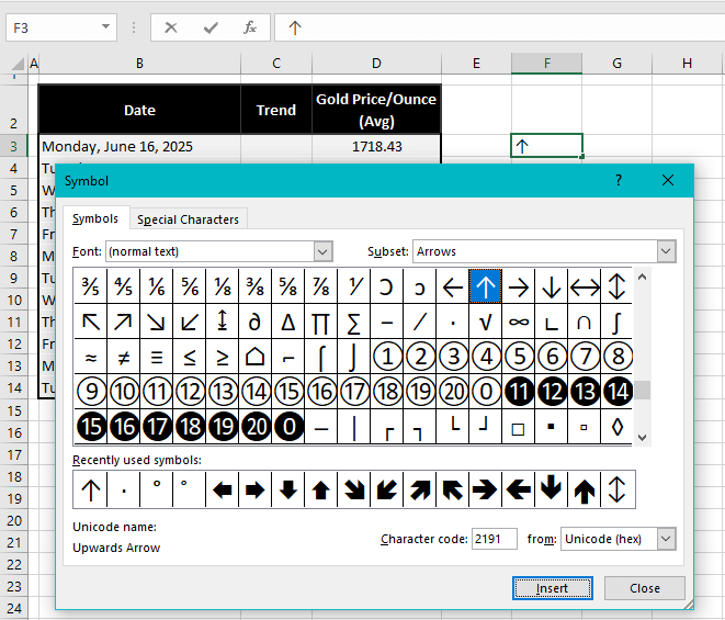
• The dialog box will remain open but in the background, the chosen symbol will be added to the selected cell on the worksheet.
• 
• Further add symbols if you wish to use more.
• Then close the Symbol dialog box with the Close
• 
• The symbol is entered in cell edit mode.
• Click any other cell on the worksheet or press the Enter key to leave cell edit mode.
• If you have inserted multiple arrows in the cell, you can copy them in cell edit mode and paste them to other cells.
• 
• Enter an IF formula to insert the arrows according to the cell values.

The arrows that we retrieved from Symbol will be added in the dataset:

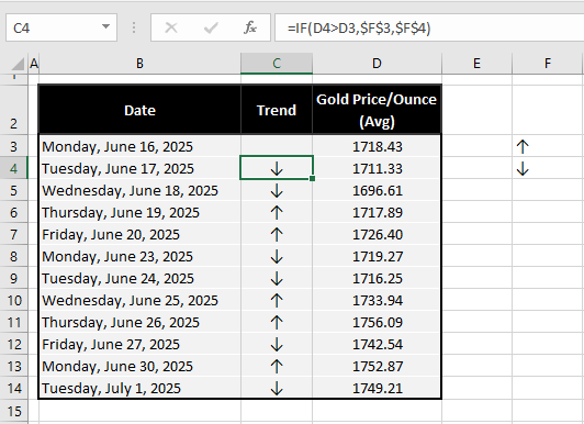
That was what we could get using a normal font. If we change the font to a symbol or special font, we open up even more types of arrows available to us. As an example, we'll show you what you can find using the Wingdings 3 font in Symbol since it is arrow galore:

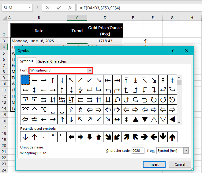
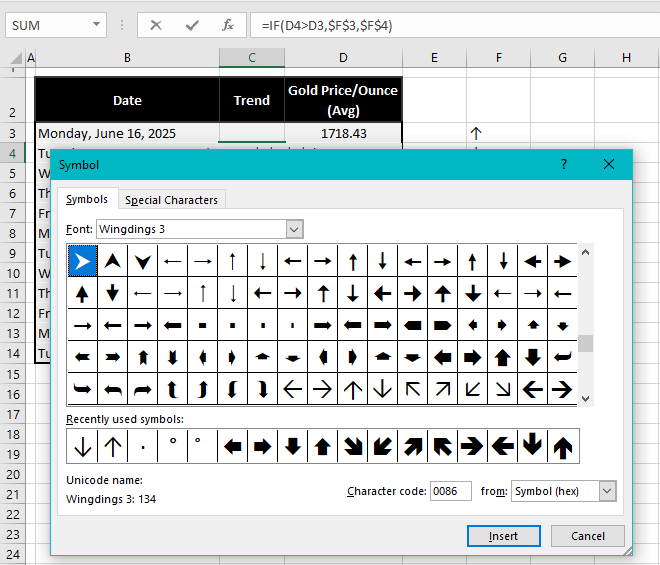
In the fourth row, you can see some hollow arrows with shadows. Simple hollow arrows can be found with the Wingdings font. Here's more from Wingdings 3:

Notes:

As we had done in copy-pasting, the arrows can be directly added to the formula from Symbol. While typing the formula, open the Symbol tool when you need to insert the arrow. Add the arrow, close Symbol, and continue to type the formula.

With a special font, the symbols don't transfer well using a formula or a value paste and you will be seeing an odd character instead of the arrow. Just change the target cell's font to the special font the arrow is from (use the Font bar on the Home tab for this) and this should return your arrow!

The reason is that inserting the arrow using a special font (let's say Webdings font) in Symbol automatically changes the font of the cell into Webdings. But when you use a formula or paste the value of the arrow, you only get the character behind the arrow.

Changing the font to Webdings (or whichever font you have used in Symbol) will immediately fix this problem. 

Method #3 – Using Shapes Option

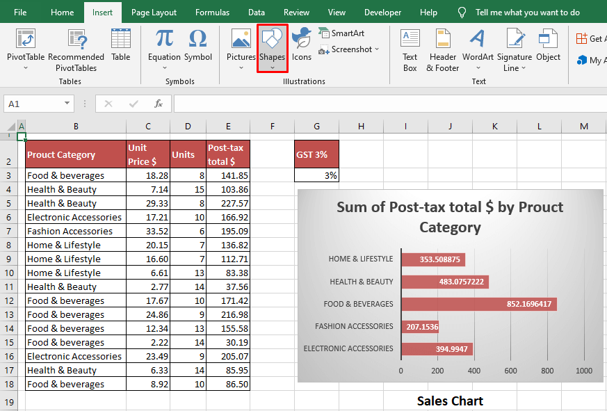
Another flexible way to add arrows is the Shapes option. Shapes offers predesigned shapes, ready to be drawn on the worksheet by clicking and dragging the mouse– far niftier than anyone's luck at freehand. Our interest lies in the arrows we can get from Shapes so let's have a look at what we need to do to insert arrows on the worksheet using this feature.

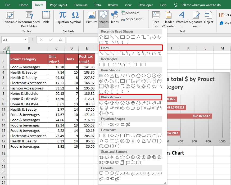
• Go to the Illustrations group in the Insert tab, and click on the Shapes icon to open the menu.
• 
• Select an arrow shape of your preference from the menu.
• The Lines and Block Arrows section have all the arrows you may need. We're adding a rightward block arrow (first arrow in Block Arrows) for our example case.
• 
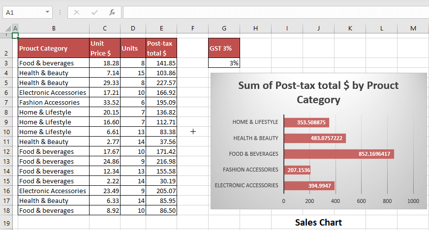
• Your mouse pointer will turn into a plus-sign cursor which is like a pen for the shape you want to insert.
• 
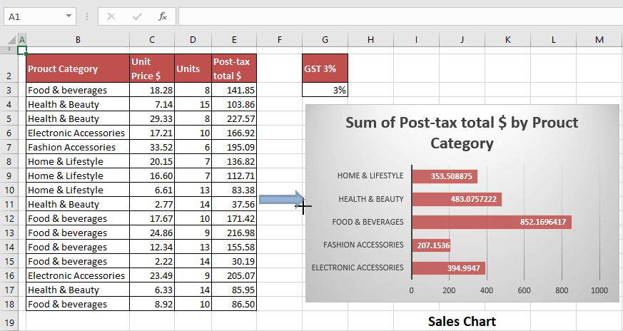
• Point the cursor where you want the arrow, and click-drag the left mouse button to draw the arrow shape (it's alright if the aim is off, you can resize, relocate and reposition the shape later).
• 
• Adjust the style of the arrow from the Shape Format

This tab appears when the inserted shape is selected.

That's all you need to do with the Shapes option to add an arrow!

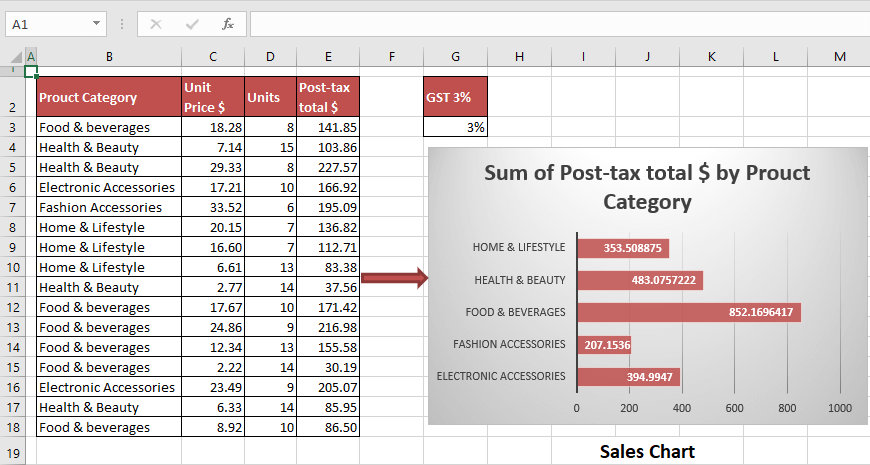
Note: The Shapes feature would be very inconvenient to use in a dataset like our previous case example with gold rates. That is because when you insert the shape, it is inserted as an object that sits above the worksheet.

Therefore, it is not a part of a cell's value and cannot be used as part of a formula. This means that every arrow will have to be copy-pasted. Why do that when other options can take care of automating the process? Still hung up on wanting colorful arrows like this for your data?

The next section will cover that for you.

If you need your arrows to do the talking, neighboring the Shapes option is another feature called SmartArt that will add more interactive arrows in your data and you can use this for objects like lists, processes, cycles, relationships, etc.

Method #4 – Using Conditional Formatting

Conditional Formatting holds the answer to so many manual Excel woes. This feature uses colors, icons, or bars to change the display of cells according to their value. You see where we're going with this? How about we try to get Conditional Formatting to display arrows, the colorful kind, according to the numeric value in the cell? Check out the steps ahead where we apply Conditional Formatting to insert arrows in Excel:

We're going to switch up our case example a bit. Let's carry forward the example involving gold rates and assume a seller's point of view. So that when gold rates would drop, that is negative for the seller and the increase is positive. The steps begin:

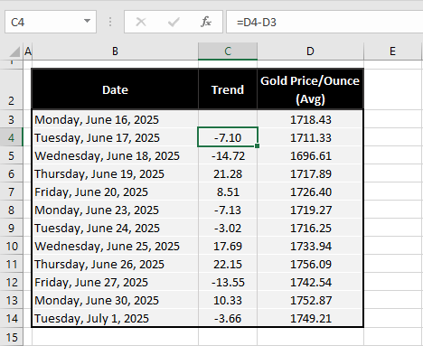
• In the column where you want to display the arrows, enter a formula calculating the difference of the prices with the preceding day e.g. =D4-D3 gives us the difference between the prices of the 16^th and 17^th of June.
• Fill the column with this formula.
• 
• Select the cells with the formula (these are the values that the arrows will replace).
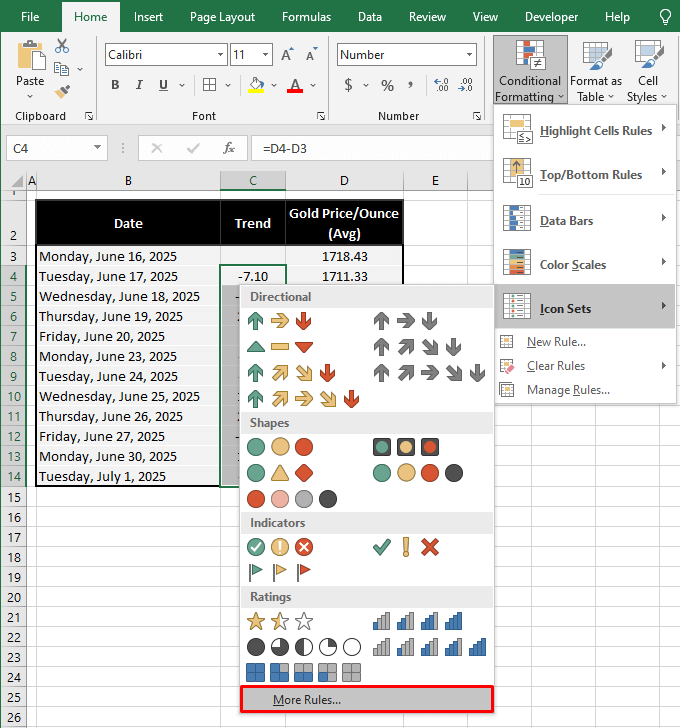
• Open the Conditional Formatting menu from the Home tab's Styles Point to Icon Sets in the menu and select More Rules.
• 
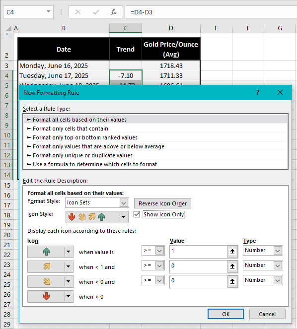
• Make these changes in the New Formatting Rule dialog box:
• Choose the arrow style from the Icon Style drop-down menu.
• Check the Show Icon Only checkbox (this replaces the cell value and displays the icons otherwise the icons appear with the values).
• In the Type section, change all three fields to Number instead of Percent.
• Change the first value from the Value section to 1 instead of 0.
• 
• Hit the OK button when done.

The arrow icons have been applied to the data. Where the price is lesser than the previous price, Conditional Formatting has displayed a red arrow and for an increase, it displays a green arrow.

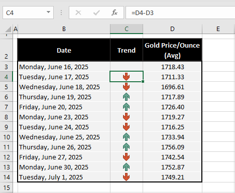
Note: Conditional Formatting does not allow relative references in Icon Sets, Data Bars, and Color Scales so you won't be able to have the arrows displayed in column D in this scenario. However, if the arrows were to be added against a fixed number or an absolute reference, they could be displayed in the same cells as the values.

Method #5 – Using Custom Format

This is another pretty cool Excel trick and we'll show you how to make it even cooler. Not only can you use a custom number format to display arrows in cells, but you can also have the positive figures appear green and the negative figures appear red. Fancy! If that's a tad too fancy for you, we'll also show you how to display arrows in a cell without changing the font color.

Do take note that this will not add an arrow in a cell and therefore it won't alter the cell's value; this is a format and will only display the arrow, keeping the value intact so the numbers can be used further in number formulas. Now would be a good time to demonstrate how to do that. Follow the steps ahead to display arrows using Custom Format.

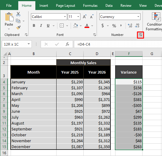
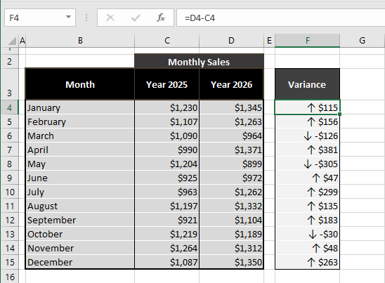
In this case example, we have a simple monthly sales report for the years 2025 and 2026 with the variance per month calculated.

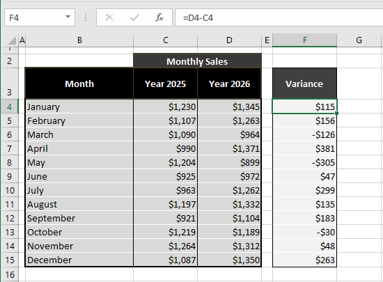
We aim to display arrows in the variance column so, go through the steps below to do the same for your work:

• Select the target cells for the arrows. We've selected the cells with the variances i.e. F4:F15.
• Click on the Number group's dialog box launcher.
• 
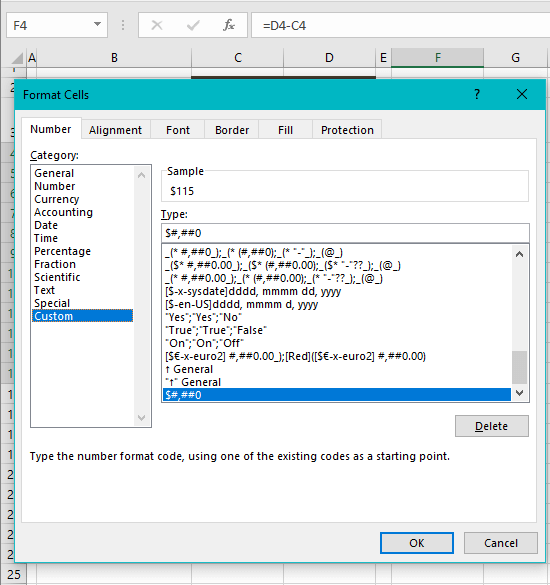
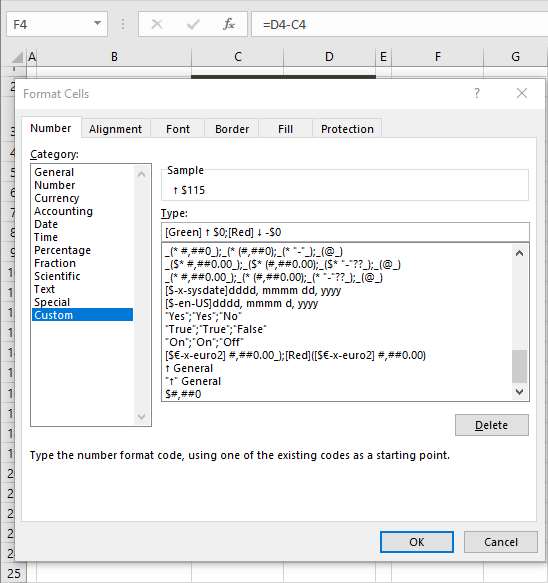
• The Format Cells dialog box will be launched with the Number tab open. And if you head to the Custom category on the left, you will see the current format of the selected cells:
• 
• This is the format we want to change.
• In the Type box, replace the current format with this custom formatting code:
• For displaying arrows without changing the font color:
• ↑ $0;↓ -$0

  We have copy-pasted the arrows in this formatting code. As per the code, a positive number will be displayed with an upwards arrow and a negative one with a downwards arrow. Applied to the selected cells, this is how it turns out:But we were talking about some color splash, remember? Use this formatting code instead if you want green and red arrows:

• For displaying green and red arrows for positive and negative values respectively:
• [Green] ↑ $0;[Red] ↓ -$0

  This formatting code displays the arrows as well as formats the font color of positive values as green and negative values as red. The Sample field will give you a preview of the format when it recognizes the formatting code.

• Select the OK button to apply the format to the selected cells.

Arrows and font colors aptly formatted:

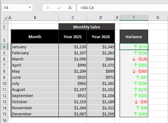
Neat!

Note: The font color set in the formatting code cannot be changed from the active worksheet.

Method #6 – Using Special Fonts

And lastly, arrows can be added in Excel using special fonts. If that sounds familiar, 10 points to you because you're right; we discussed using special fonts via the Symbol feature. Now we'll talk about using special fonts directly on the active worksheet.

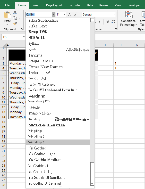
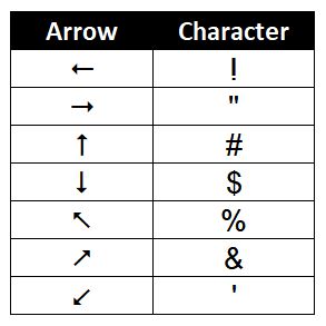
How is this going to work? You need to enter (type, paste, or insert) a character and change the font of that cell to a special font so that it returns an arrow. Which font and what character? Every special font turns a character into a different symbol. E.g. an exclamation point "!" will be a spider web symbol with the Webdings font, pencil with Wingdings, pen with Wingdings 2, and a left arrow with the Wingdings 3 font.

Taking cue from there, we'll show what characters you need for different arrows. There are many more types of arrows that can be accessed with special fonts and you are free to explore them but our suggestion below includes easy characters that you can type from your keyboard. Here's what you need to do.

• Add the character to the cell where you want the arrow.
• The characters and their corresponding arrows with the Wingdings 3 font are mentioned below:

• Font: Wingdings 3

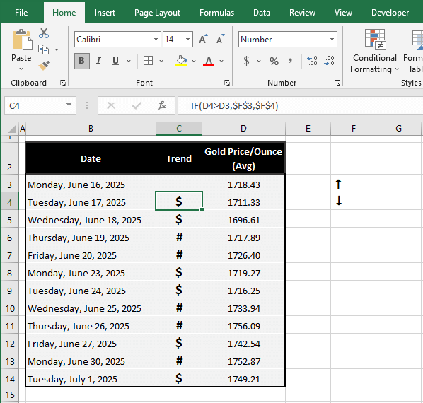
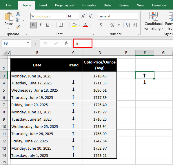
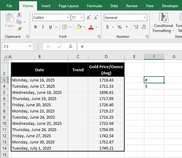
  We're entering a number sign "#" in cell F4 and a dollar sign "$" in F5 to get the up and down arrows.Select these cells and change the font to Wingdings 3. This won't change the font of the results of the function but this way you can confirm if you're putting the right character through.
• Enter the formula in the cells where you want the arrows.
• You should be seeing the characters (number and dollar sign in our case example) as the formula's results.
• 
• Select the characters and change the font to the respective special font (Wingdings 3 for us).

You should successfully have the arrows in place!

The Formula Bar displays the character when you select the original arrow and the special font can be viewed in the Font bar. As a cell value, the arrow can remain in the special font while other characters and values can be added in the same cell in regular fonts:

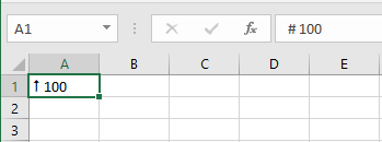
The pro? You won't have to access any other feature for the arrows. The con? You still need to know which character will return what arrow.

That's all there's up with inserting arrows in Excel. All the methods add arrows to the cell value except for the Shapes option which inserts the arrow above the worksheet and the Custom Format which only displays arrows. Arrows (as text values) can be used as part of formulas and formatting codes. We hope we've "pointed" you in the right direction.