How to Select Every Other Row in Excel (3 Quick & Easy Ways)

To work on every other row in Excel, you would have to select them first. A continuous selection is no problem at all but selecting alternate rows? That doesn't need to be a problem either even though Excel does not have an explicit alternate row-selecting feature.

Deleting or highlighting every other row and deleting or copying their data are some instances where you would need to select alternate rows. Consider a small example of randomly selecting names from a list and the choice of selection is every other row.

As a side note, if your only focus is on highlighting every other row, selecting them is not a prerequisite and this can be done directly through Conditional Formatting.

Our tutorial today details 3 easy ways of selecting every other row in Excel. Outline your objective and select the method that best suits it. Manually selecting the rows selects the full row on the sheet and is best for small datasets.

Selecting rows with a helper column or VBA gives the user discretion in how much of the row is to be selected and should be the go-to choice with larger datasets.

With the broader descriptions covered, we're ready to explore all the Excel tricks for selecting every other row.

Get set select!

Method #1 – Manually Select Every Other Row

Every other row in Excel can be selected manually. We know what you're thinking; manually? But is there really any point in whipping up a function or picking out a code if you just need to select, let's say 5 rows? Or even 10.

That won't be working fast or smart so adopt this option if there's a very small lot to be selected and if you want to select the full row instead of the rows within a dataset. So if that is the situation and you agree with us, you can select alternate rows manually.

Selecting every row goes the same way as making multiple noncontinuous selections on your computer, clicking while holding the Ctrl key. The steps ahead offer the complete details of manually selecting every other row in Excel:

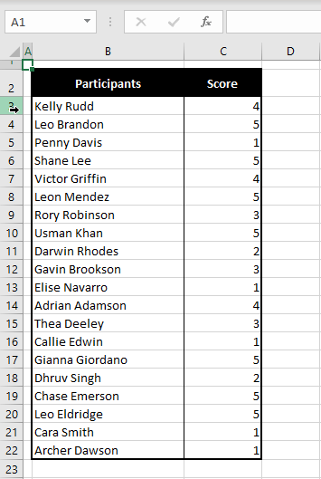
• Point the cursor to the row header of a row that you want to select. The cursor will show as a rightward pointing arrow.
• In the example below, we are pointing to row 3.
• 
• Click to select the row.
• Press the Ctrl key and keep it held down as you point the cursor to the next alternate row's header and click again.
• Our next selection will be row 5.
• 
• Keep the Ctrl key pressed as you click and select all the rows.
• When done, let go of the Ctrl

Every other row within the dataset will be selected:

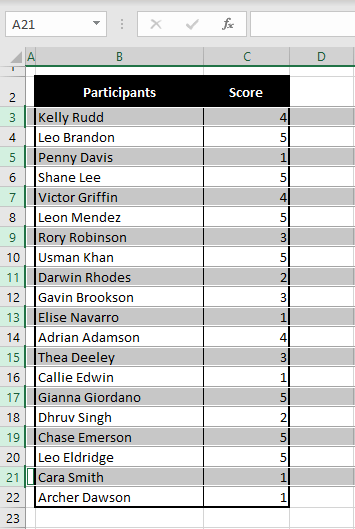
Note: Selecting the rows manually by clicking on the row headers selects the entire row, not just the rows in the dataset.

If you prefer to keep the selections limited to the dataset, the other two methods in this tutorial should help you fine.

Method #2 – Using Helper Column

Select every other row in Excel using a helper column. By a helper column, we would enter true and false values, filter one of them out, use the Go To Special feature to select the visible cells and we should be done.

The benefits of selecting rows this way? The prime one is that it is far less manual than selecting rows manually; with several clicks, alternate rows will be selected automatically. This brings us to another point, automatic selection leaves out the chances of human error that can be made while selecting manually.

Third, the selection of the rows can cover as many or little columns in the data set without selecting the entire rows as we have seen in the previous section. Follow the steps below and you will be able to select every other row in Excel using a helper column:

• In a free column adjoined to the dataset, add any header (as we have added "HELPER" in our example).
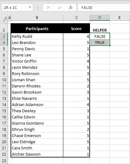
• Enter "TRUE" and "FALSE" in the first two rows of the helper column. Any order is fine.
• Select both these values (we have selected cells D3 and D4).
• 
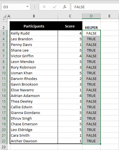
• Use the Fill Handle (small green box at the bottom-right corner of the selection) to fill the column in line with the dataset (filled to D22 in this example).
• Now the helper column is populated with alternating TRUE and FALSE values.
• 
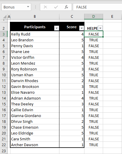
• Select any cell within the dataset or the helper column and press the Ctrl + Shift + L keys to add filters to the data. The clickable option for adding/removing filters is the Filter option in the Sort & Filter menu (Home tab > Editing group).
• The headers of the data will now end with small drop-down arrows that are column filters:
• 
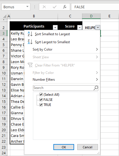
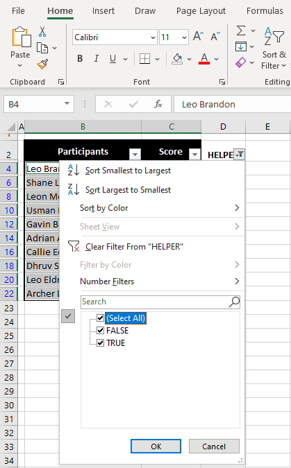
• Select the filter arrow of the helper column.
• The filter shows that currently, both TRUE and FALSE values are displayed:
• 
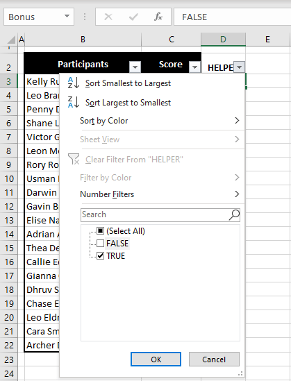
• Uncheck the FALSE box.
• This will remove all the rows with the FALSE value in the helper column and we will be left with all the rows with the TRUE value. The first TRUE value is in the second row of the dataset so if you prefer to start the selection from the first row, you can uncheck the TRUE box instead of FALSE.
• 
• Now click on the OK
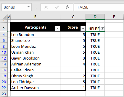
• All the rows with the FALSE values in the helper column have been filtered out and the TRUE ones are displayed. How symbolic.
• 
• Select the range from the remaining dataset.

In this example, we are selecting all of the remaining dataset. If your dataset has multiple columns, you can select the amount you prefer and can even make a discontinuous selection (e.g. selecting columns B and D of a dataset).

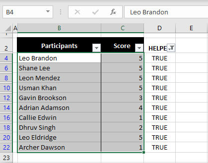
Now if you want to copy and paste this selection somewhere, you can go right ahead. This is what pasting our selection looks like and it only contains the data from the alternate rows, put together:

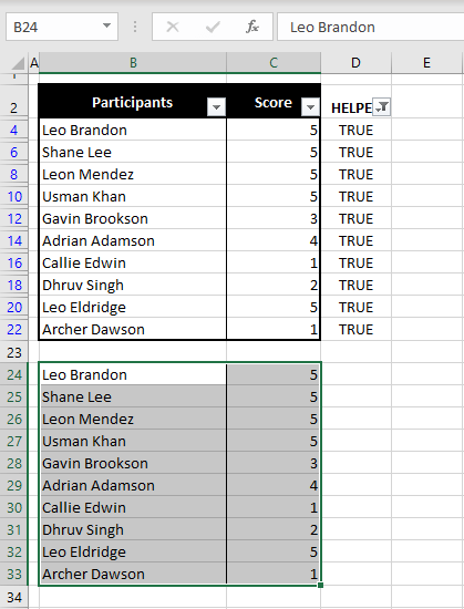
But without pasting it anywhere, if you unravel the dataset back to its full form, the selection of alternate rows doesn't remain:

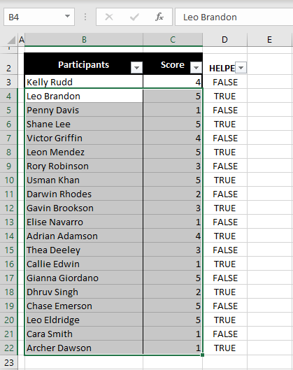
For the alternate rows selection to remain when the whole dataset is restored, we will need to select the visible cells while the data is filtered. So, let's go back to the state of the filtered data from where we can proceed:

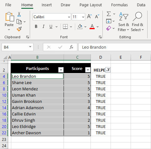
We have the rows with TRUE in the helper column displayed and we have selected the remainder of the dataset.

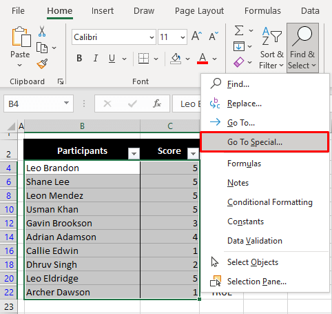
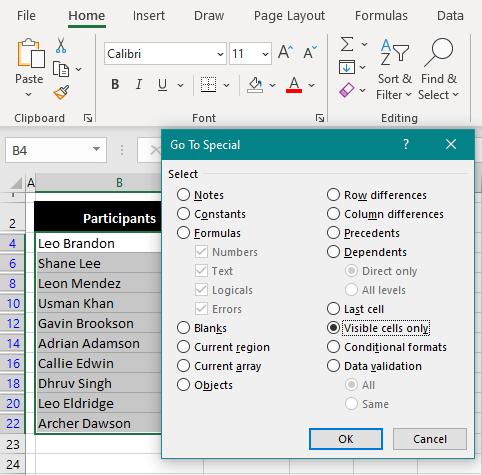
• In the Editing group of the Home tab, click on the Find & Select icon and select Go To Special.
• 
• In the Go To Special dialog box, choose the Visible cells only radio button.
• 
• Then select the OK
• The dialog box will close, selecting the visible cells from the filtered rows. The change in the selection is notable with breaks along every row. The breaks signify hidden rows.
• 
• Now open the helper column's filter again and restore the dataset by selecting the Select All
• 
• Click on the OK

The dataset in complete display will reveal that every other row is selected:

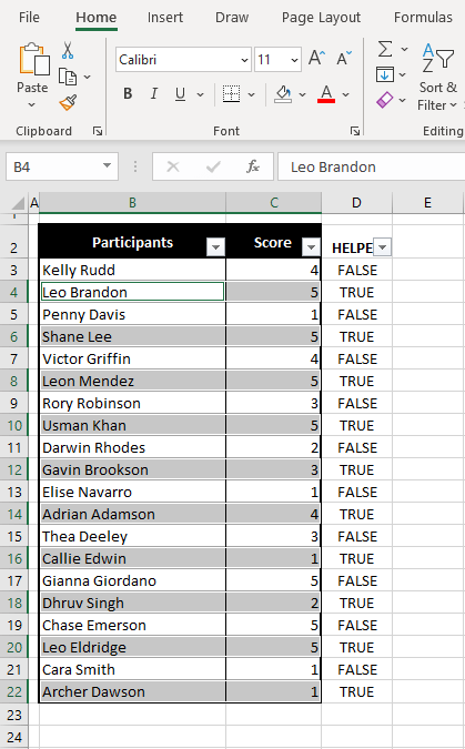
Once you are through with the intended task for selecting every other row, you can delete the helper column.

Notes:

The alternate TRUE and FALSE values are added for selecting every other row. You can change the pattern for selecting every Nth row. E.g. for every third row, you can enter FALSE FALSE TRUE and populate the helper column with that pattern.

The TRUE and FALSE values can also be entered by using either the ISEVEN or ISODD function (along with the ROW function). These will return TRUE and FALSE according to the row numbers. But using these functions will limit the selection to every other row only and not every Nth row.

Method #3 – Using VBA

Use VBA to select every other row in Excel. VBA is used in Microsoft applications to automate tasks.  With VBA, a code can be run that loops through the selected data to select alternate rows. We have elaborated on this matter in the steps listed ahead. The steps for selecting every other row using VBA in Excel:

• Select the columns of preference in the dataset.
• We have selected columns B and C.
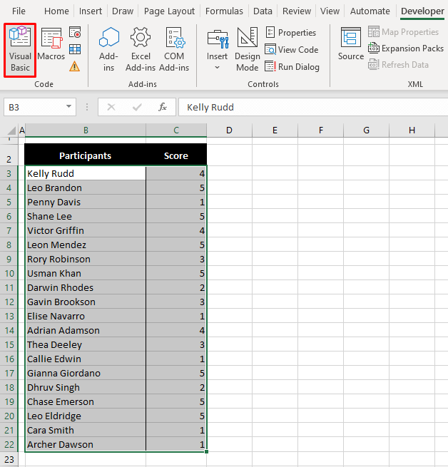
• With the Developer tab, it will be easy to select the Visual Basic button to launch the Visual Basic editor, but you can also accomplish that with the Alt + F11 keyboard shortcut.
• 
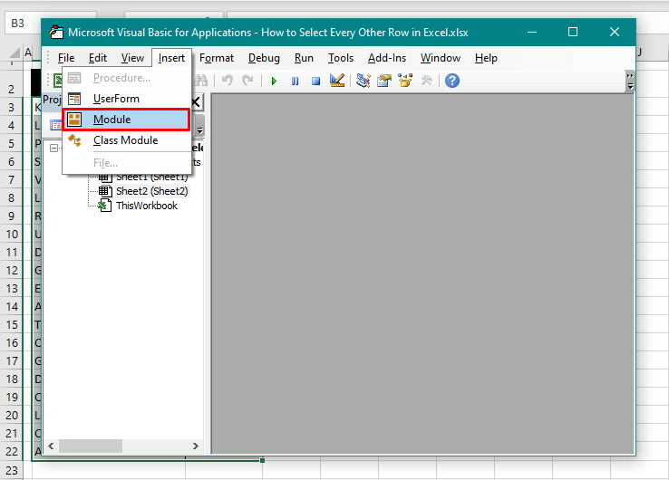
• In the Visual Basic editor, click on the Insert tab and select the Module
• 
• A Module window will open.
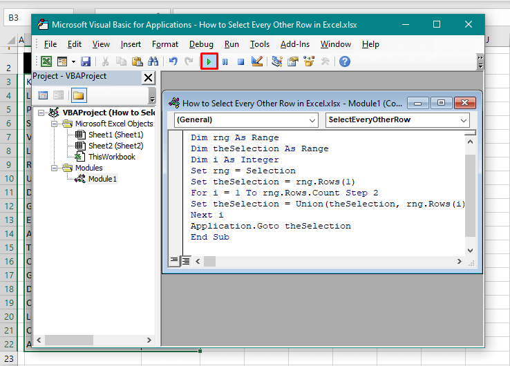
• Copy the code below and paste it into the Module window:

• Sub SelectEveryOtherRow()
  Dim rng As Range
  Dim theSelection As Range
  Dim i As Integer
  Set rng = Selection
  Set theSelection = rng.Rows(1)
  For i = 1 To rng.Rows.Count Step 2
   Set theSelection = Union(theSelection, rng.Rows(i))
  Next i
  Application.Goto theSelection
  End Sub

  This code will select every other row starting from the first row of the selection. This is because of the values in lines 6 and 7 of the code. The current values are:

  Set theSelection = rng.Rows(1)
  For i = 1 To rng.Rows.Count Step 2

  The number 1 in both lines of the code starts the selection from the first line. Step 2 in the 7th line defines the step in the selection (every alternate row). Change this to N for every Nth row (e.g., 3 for every 3rd row) and change the 1 in both lines to the number where the first selection is to begin.

• When done entering and adjusting the code, click on the Run button as highlighted above or hit the F5 key to run the code.
• The code will be run in the background of the editor and will select every other row. You can leave the editor open, reselect the dataset, adjust the code, and run it again if you want to make a different selection.
• When you are satisfied with the selection, close the Visual Basic

Here is the selection of every other row using the above-mentioned code in VBA:

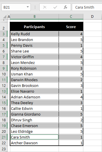
There are plenty of ideas for selecting every other row and Nth row in Excel. We'd be happy to dish out more Excel ideas and troubleshooters while you're testing today's lesson. Who'll beat who? Ready? Tricky? Go!