How to Select Only Visible Cells in Excel (Shortcut + VBA)

Does not sound like an issue, right, because how would you even select cells that aren't visible? You would and that is no magic or the lack of it; that's just a very regular way of Excel. A demonstration you say? Good idea. Let's show you how you'll end up selecting hidden cells with an example. Below we have a dataset of product quality scores out of a total of 20.

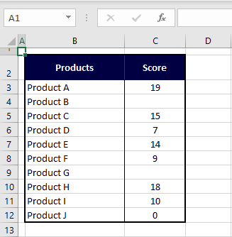
The scores regarding some of the products haven't come in yet so we'll hide those rows for now.

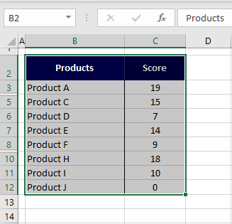
You can now see that rows 4 and 9 are hidden, also hiding products B and G. The breakpoints in the row headers indicate hidden rows:

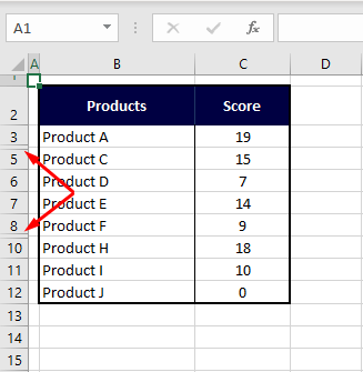
What do you think will happen if we attempt to copy-paste only the dataset shown above? Will the hidden rows be copied or not? For testing, we pasted the data right below the original dataset:

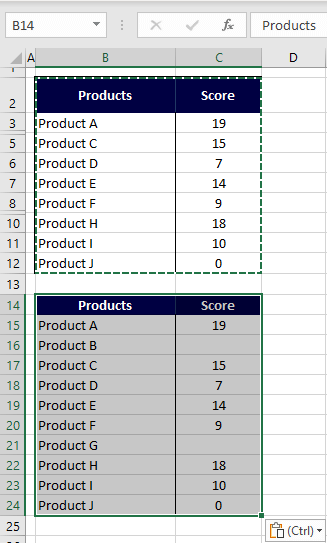
The original dataset has been copied as it is including the hidden rows. Why has that happened? When the cells were selected, even with the rows hidden, the selection actually is B2 to C12. That, therefore, includes the hidden rows and would also include hidden columns, if any.

So, what are visible cells? Visible cells are those not hidden by way of hiding rows and columns. In our case example, we are referring to the visible cells within the dataset. Rows and columns are hidden to make data concise due to the volume or when some of it is irrelevant.

Back to the question that started all of this – how to select only the visible cells, leaving out hidden rows and columns? There are a few very quick ways of doing that which are the Go To Special feature, a keyboard shortcut, the Quick Access Toolbar command, and VBA.

Let's get visibly selecting!

Method #1 – Using Go To Special Feature

Select the visible cells of a set of data in Excel with the Go To Special feature. Go To Special finds and selects cells of a specific characteristic depending on the selected cell or range. The characteristic useful to us right now is visible cells. The following steps contain the method of selecting visible cells using the Go To Special feature:

• Select the dataset from which you want the visible cells to be selected.
• 
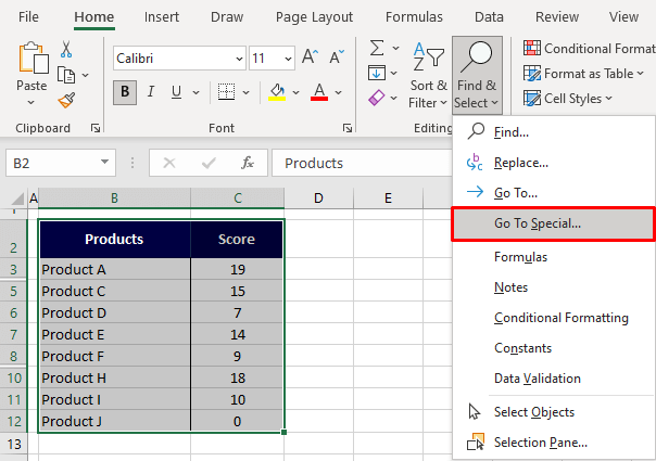
• Click on the Find & Select button (located in the Home tab's Editing group and select Go To Special.
• 
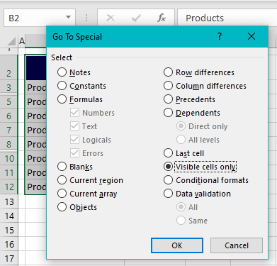
• The Go To Special dialog box will open.
• Select the Visible cells only radio button.
• 
• Then click on the OK

The dialog box will close and back to the sheet, the visible cells will be selected without the hidden rows and columns:

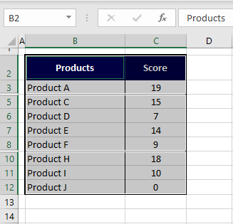
Can you tell the difference by looking at the selection above? If you can't then look below:

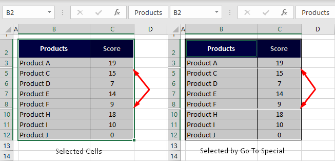
Selecting the dataset normally shows a smooth gray selection. Selecting visible cells shows breaks in the selection where the rows and/or columns are hidden. Using this selection, if we now copy-paste the dataset, it will be devoid of the hidden rows/columns:

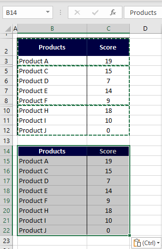
It works! The pasted dataset does not include the hidden rows of products B and G. The path to using Go To Special for selecting visible cells can be made into a keyboard shortcut but it would contain thrice as many keys as the shortcut below so, check it out!

Recommended Reading: How to Only Sum Visible Cells in Excel

Method #2 – Using Keyboard Shortcut

Visible cells in Excel can be selected using a keyboard shortcut. The keyboard shortcut is:

Alt + ; keys

To apply the keyboard shortcut, follow these steps:

• Select the data.
• 
• Press the Alt and semicolon ( Alt+ ; ) keys.
• The keyboard shortcut will leave out the cells of the hidden rows/columns and select the visible cells in the selected data:

That was the quickest way of using the keyboard.

Method #3 – Using Quick Access Toolbar

And this could be the quickest way of using the mouse. From the Quick Access Toolbar (QAT), the visible cells of a dataset can be selected in Excel. Once the shortcut is added to the Quick Access Toolbar, the action is just a click away. See how to add the Select Visible Cells command to the Quick Access Toolbar and then how to use it on a range.

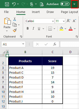
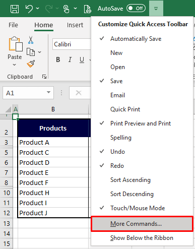
• Click on the Customize Quick Access Toolbar arrow in the title bar.
• 
• Select More Commands from the list.
• 
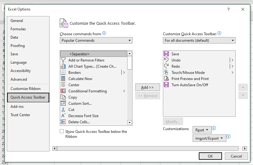
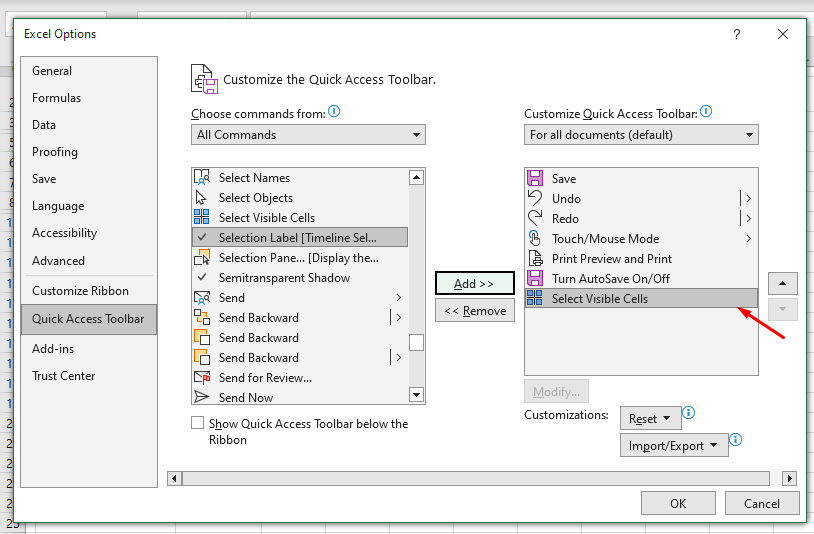
• You will be redirected to Excel Options which at this point will look like:
• 
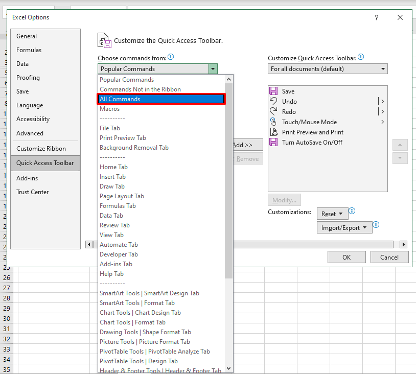
• From the first drop-down menu, which reads Popular Commands, select the All Commands
• 
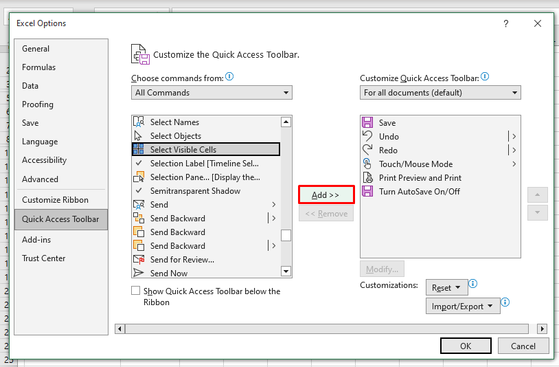
• In the list below, scroll down to the S section and choose the Select Visible Cells
• Or you can click on any command and start typing the command name and then select it.
• Next, use the Add button from between the two lists to add the command to the Quick Access Toolbar.
• 
• After the Add button, the command will be enlisted in the list on the right.
• 
• Press the OK button to close the dialog box after the changes.
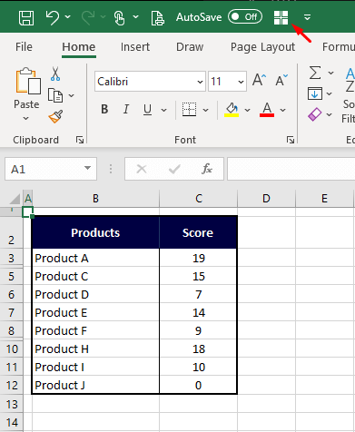
• The added command will show in the title bar, at the end of the Quick Access Toolbar:
• 
• To use the command, first select the range on the worksheet. For us, that is B2:C12.
• Then click on the Select Visible Cells command from the Quick Access Toolbar.

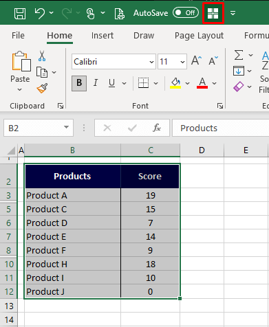
The command will alter the selection to only the selection of the visible cells:

Method #4 – Using VBA

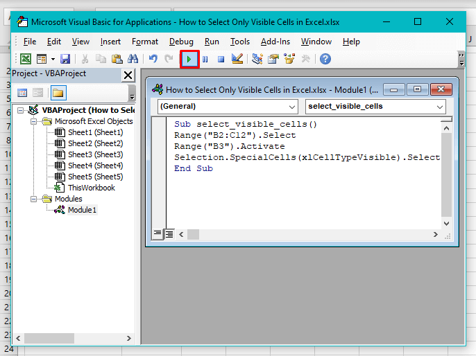
Lastly, VBA can come into play for selecting visible cells in Excel. VBA automates Excel tasks with user-defined codes. We will also use such a code to select the visible cells from the chosen range. The steps below will guide you on how to enter the code with VBA and use it to select visible cells:

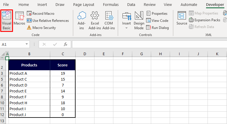
• Go to the Developer tab > Code group > Visual Basic The button will lead to the Visual Basic editor (also accessed by the keyboard shortcut Alt + F11 keys).
• 
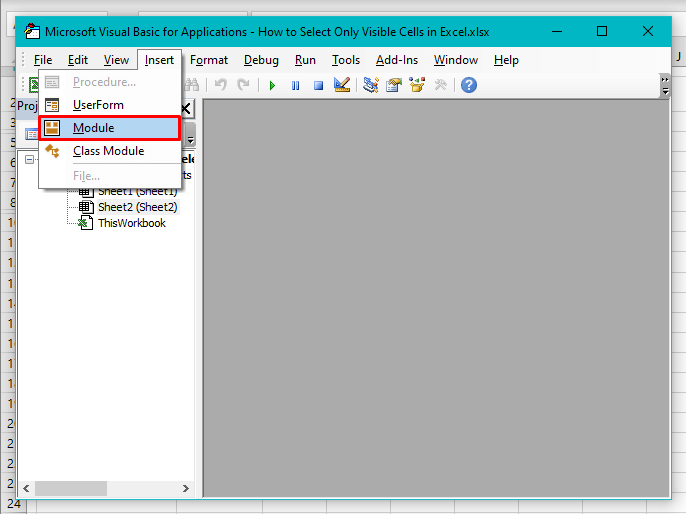
• In the editor, select the Insert tab on the top and then select Module from the Insert
• 
• You should see a Module window appear.
• Copy and paste the below-mentioned code into the Module window you just opened.

• Sub select_visible_cells()
  Range("B2:C12").Select
  Range("B3").Activate
  Selection.SpecialCells(xlCellTypeVisible).Select
  End Sub

  Edit the code for the range you want to apply it to. B2:C12 in the second line of the code is the range that will be selected on the worksheet. B3 in the next line is the point from the selection of visible cells that will be activated.

• When done, hit the Run button (or the F5 key) to run the code.
• On the worksheet in the background, the code will select the visible cells from the range B2:C12.
• Close the Visual Basic

And find the visible cells selected from the data range supplied in the code:

Did you already know how to do that? So where are you heading next; to your spreadsheet to finally just select the visible cells or to another Excel trickery? Ready? Tricky? Go!