#SPILL! Error In Excel – How To Fix

#SPILL! error in Excel is most commonly experienced while using a dynamic array function. A formula that cannot fill the required cells with the calculated results creates this error.

After the introduction of dynamic arrays, the formulas can often return multiple values. In such cases, the result will be "spilled" in the worksheet, and the cell range is known as the "spill range".

The most common scenario of the #SPILL! error is when there is a spill range blockage or the reference used for the formula is beyond the limits of the worksheet.

In this tutorial, we’re going to walk you through what the #SPILL! error is, why it occurs, and the ways to fix it.

What is a #SPILL! Error in Excel?

A #SPILL! error typically happens when a formula generates several results but cannot output them on the worksheet. To better understand the error, you must first understand the terms such as 'spilling' and 'spill range'. Along with the cell obstruction case, there are several other cases where you might face the  #SPILL! error in Excel.

We are quite accustomed to entering a formula, receiving the result in the same cell, and then extending that formula by click-and-drag. But what would happen if only one entered formula is to produce more than one result?

The term "spill" describes the behavior in which formulas that yield numerous results automatically "spill" their results into numerous cells. The result will be spilled in the worksheet taking up the required number of cells to display the result. E.g. if one formula needs 5 cells to display its result, it will fill 5 cells including the cell the formula is in.

The range of values that an array formula returns and spills into a worksheet is called the "spill range".

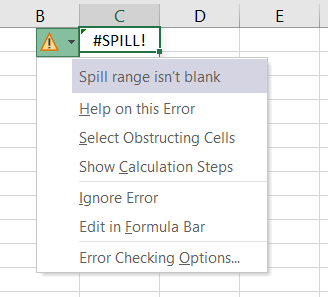
It is usually highlighted with a dashed blue border. Excel also helps you understand what went wrong with your formula. If your formula brings about an error, selecting the cell will display an error icon. Click this icon to get help with the error along with access to more options on handling the error.

Reasons for #SPILL! Error in Excel

Below mentioned are several possible causes of #SPILL! error along with their fixes.

1- Spill Range is Obstructed

This is one of the most common and basic cases of  #SPILL! error. There is no space on the worksheet to show the return values. For example, if the formula is expected to return two values, but only one neighboring cell is available, it will give a #SPILL! error.

The error will vanish after removing the obstruction, and the range will be filled with the predicted formula results.

Example 1 – Spill Range is blocked

In our example, we have a list of names that are split into first and last names in columns A and B. If we are to re-organize the data from a vertical to horizontal set, one way to do that is to use the TRANSPOSE function. This formula would do for transposing the list in column A to row 1:

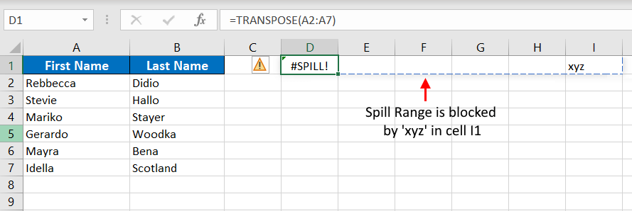
To rearrange the data, we’ve supplied the TRANSPOSE function with the range A2:A7 containing the first names in column A. The formula is entered in cell D1. With 6 names in column A, the formula will need 6 cells to display and spill the result i.e. from D1 to I1.

However, because there is data in cell I1, the spill range is blocked. Hence the #SPILL! error.

Solution 1: 

The first instinctive solution for this #SPILL! error is to remove the obstruction which is to delete or move the data from I1. When the data is deleted, the result of the formula will spill to I1 – #SPILL! error taken care of!

However, it may not always be possible or convenient to get rid of the data and so you have another option to fix this error.

Solution 2:  

The other solution is to relocate the target cell of your formula. Since the spill range ahead of D1 has a non-blank cell, there is no issue in this scenario to move the formula a few cells down. Therefore, we have shifted our target cell from D1 to D5 which allows the result to spill freely to I5.

There can be several other instances where you might face a similar issue. The blocked spill range can be due to value, a special character,  an invisible character, or a cell with a formula returning an empty value.

Example 2 – Invisible Obstruction

As compared to a blocked cell that we can clearly see, the error could be due to a blocked cell, that is not visible. This can be because of the font color, or because the cell data is formatted to make the cell value disappear using the custom format ;;; via the Format Cells dialog box.

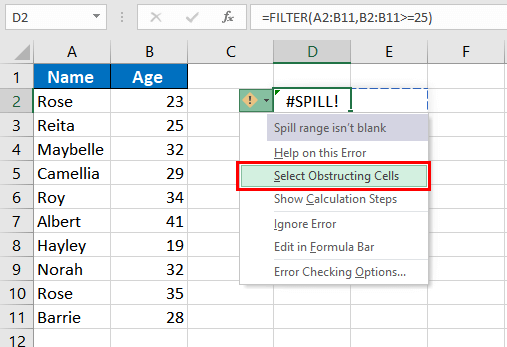
For the example below, we have the ages of a group of people and are using the formula ahead with the FILTER function to list down the people aged 25 and above:

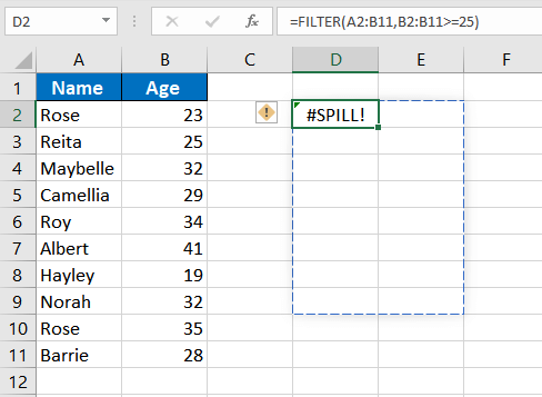
The formula is giving a #SPILL! error, but there is no visible obstruction.

Solution:

To fix it, click on the Error floatie and choose "Select Obstructing Cells". It will highlight the cells where there is data. D7 shows the text “Block”, but we cannot see it.

It is because the font is white. Remove the data, and the error is fixed.

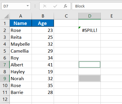
Similarly, cell D9 shows the text ‘Block 2’ with the font color black, but we are still unable to see it. It is because the cell is formatted to disappear. To check, right-click on the cell and select Format Cells. is  ";;;" If in the Number tab, you find that the Custom category is selected with ;;; in the Type box, it is a formatted cell whose value is formatted to be invisible.

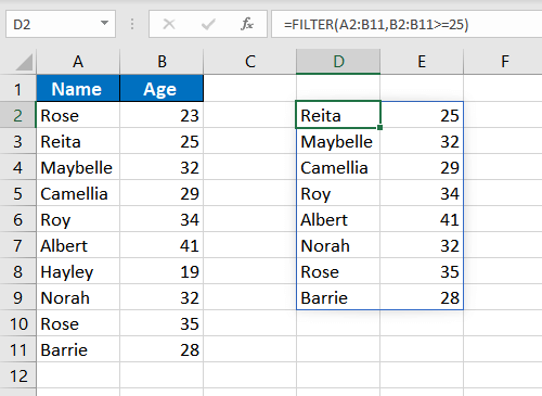
The solution is simple; either delete the value or shift the formula where there is enough space for the spill range.

2- Merged Cell in Spill Range

The #SPILL! error in Excel is also experienced if the spill range includes a merged cell. Click on the warning flag and look at the cause, "Spill range has a merged cell" to make sure that the merged cells are to blame for the problem.

Example – Spill Range includes merged cell

The example we have here has a list of products with their respective categories. To get the final range of the categories, the formula below with the UNIQUE function can be used:

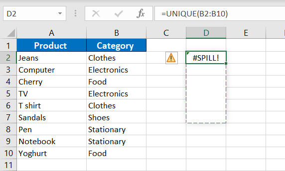
Using this formula with B2:B10 as the given range, we are trying to find unique values in the category column. There is a #SPILL! error because D4 is merged with D5 and D6; a part of the spill range.

Solution

Unmerge the cells in the spilling space by selecting the merged cell and going to the Home tab > Alignment group > Merge & Center button. If you have large data, click on the error symbol, select the Obstructing Cells option to automatically locate the problem cells, and then unmerge the problem cell.

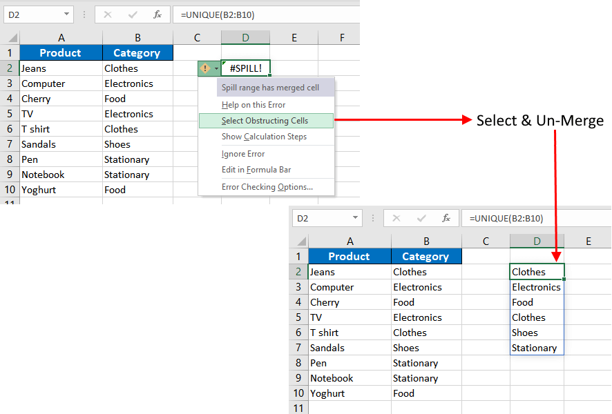
No merged cell – no problem; the #SPILL! error will be solved as the merged cell will be gone.

3- Spill Range is Undetermined

Dynamic Array formulas when combined with volatile functions such as RAND, RANDARRAY, RANDBETWEEN, etc., result in the  #SPILL! error. This is because volatile functions cause frequent recalculation.

Hence, the dynamic array formula cannot define the spill range. This will cause Excel to show ‘Spill Range is Unknown’ as the error description using the error icon.

Example – Using SEQUENCE & RANDBETWEEN

The following formula generates a #SPILL! error:

Since the result of RANDBETWEEN varies frequently with every recalculation on the sheet, the SEQUENCE function, which is to return numbers in sequence, is unsure of how many values to produce. Therefore, the spill array is unknown/can’t be determined and so Excel gives us a #SPILL! error.

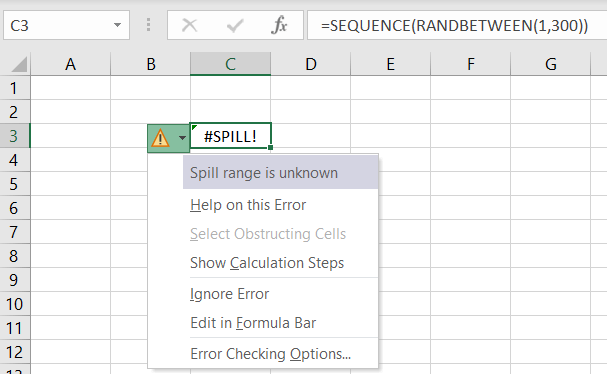
By checking the "Spill range is unknown" cautionary indicator, you can verify the error's root cause.

Solution

Sadly, the solution is to use a different formula. You can use alternative formulas that produce arrays or ranges with defined lengths.

4- Spill Range is Beyond the Limits of Worksheet

When using a formula that might return too many values for the worksheet, it will return a #SPILL! error. In such cases, the formula’s spill range is such that it would extend outside the borders of the worksheet. It can be better understood using examples.

Example 1 – The spill range is big

For the employees in this example, we are trying to increase everyone’s salary by 10%. This should be achievable with a simple formula like the one below:

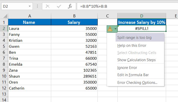
Here, column B refers to the salary column and the idea is to increment the whole column by 10%. It gives a #SPILL! error because the spill range is more than the rows in Excel. Excel contains 1048576 rows. To return the calculation on an entire column, column B in our case, the formula will require 1048576 rows.

We are using the formula in D2 and the formula will need the 1048577^th row to display the complete result. Since Excel doesn’t have rows beyond 1048576, this means that the spill range will go beyond the worksheet. That is not possible, creating the #SPILL! error.

Solution 1: 

If we use the same formula in E1, it will spill the required result. You are getting a #VALUE! error because it is also trying to calculate the value of B1 which is not a numeric value.

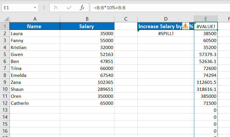
Solution 2: 

Instead of referring the whole column B:B, you can define the range that column B covers in the dataset as B2:B12 and use this formula instead:

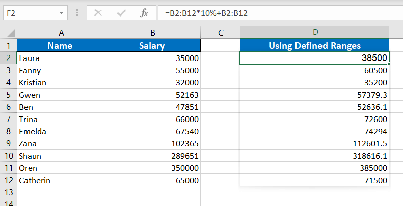
This formula will result in a spilled range from the target cell D2 to D12.

Solution 3: 

Use only the cell reference of the first row of the dataset (that is row 2 for us. For column B, the first data cell for the formula will be B2), then using the fill handle, copy the formula to your required range.

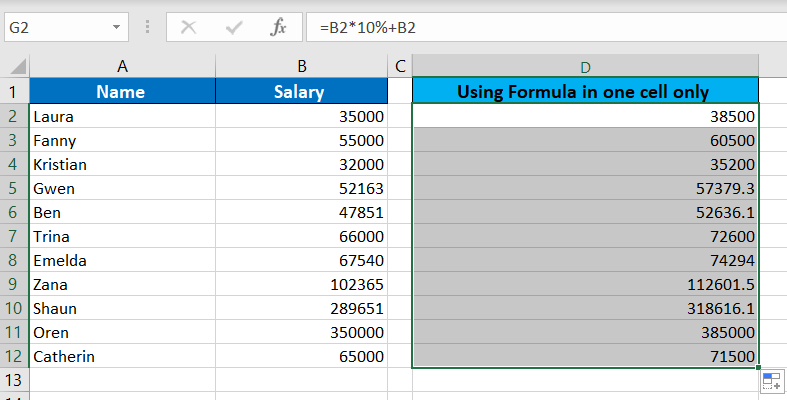
Use the formula in D2 using the reference of cell B2 only. Then drag to duplicate it to D12.

Example 2 – Implicit intersection (@)

Implicit intersection operator "@" converts an array or range to a single value. If a function exceeds the spill range to the edge of the worksheet, use "@" to convert it to a single value. Then drag and copy the formula to the remaining cells.

In the example, we are using the VLOOKUP function through this formula:

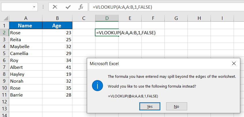
Ideally, the function will look up cell A2; but since the column reference we’ve used is A:A, it will look up the entire column A, making the spill range exceed the worksheet space. Excel itself will give an error and suggest you use ‘@’.

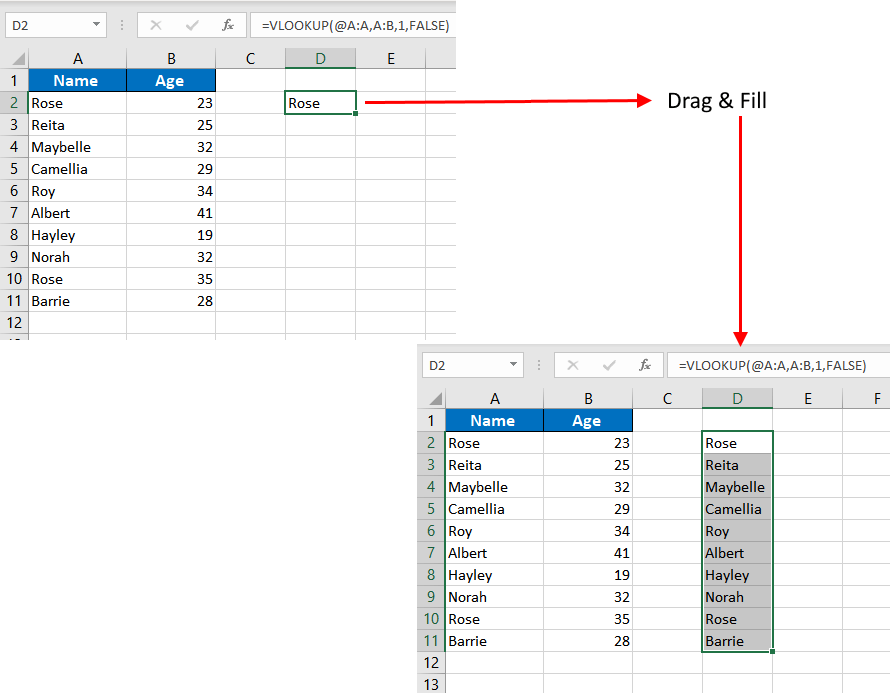
When you accept the suggestion by the prompt, it adds the implicit intersection operator and returns the value of A2 (the particular row where the formula is written). You can then drag the formula to fill and complete your range.

Example 3 – Results spilling beyond the worksheet column limits

There are 1,048,576 rows and 16,384 columns in Excel. If you use a formula that spills beyond the sheet, it will give a #SPILL! error.

If you use the above formula (or SEQUENCE function with any number greater than 16,384), it will result in a #SPILL! error.

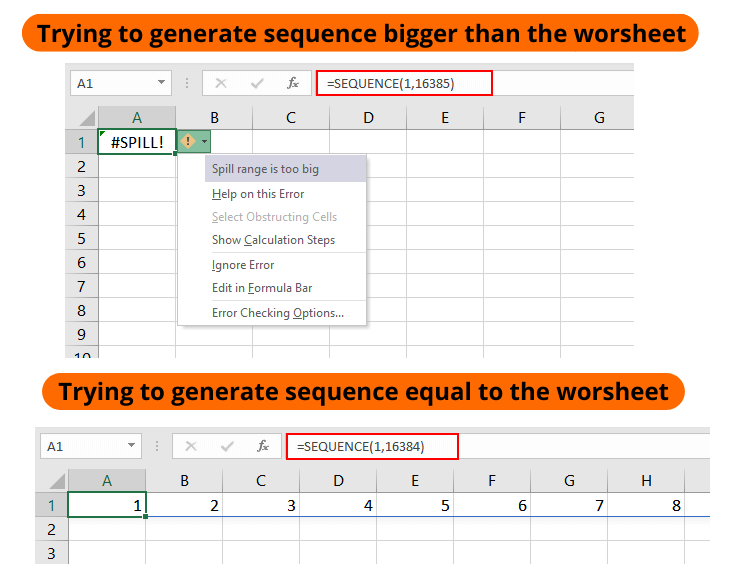
To fix this error, you can try changing the formula as:

Make sure to enter it in the first column so that it will spill your sequence all the way to the last column without needing more columns.

Solution

Avoiding references and calculations that could result in spill ranges that don't fit the worksheet or try to shift the target cell to earlier rows/columns so that the formula has enough cells for the spill range.

5- Excel Tables With Dynamic Arrays

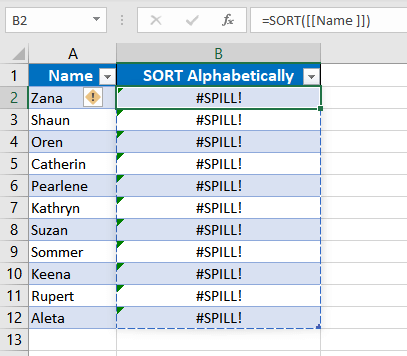
Dynamic array does not work well with the Excel Tables. If you try to use an array formula within a table, it will result in a #SPILL! error. To verify the case, check the error symbol that shows ’Spill range in table’.

Example – Array Formula in Excel Table

The example comprises a list of names in an Excel Table. Now we’ll use the following formula so the Name column is sorted in alphabetical order.

We have encountered the #SPILL! error again. With the target cell in selection, we can click on the error icon to confirm the reason for the #SPILL! error which is ’Spill range in table’.

Solution 1

Use the formula outside the Table referring the Table and column. Copying the formula from above, we’ve referred the Table name in the formula:

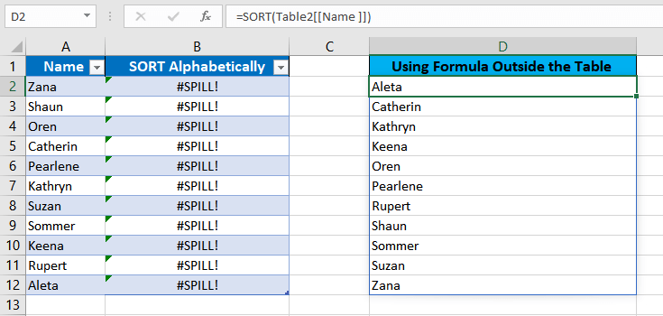
If the formula is placed in F5 instead of D5, it shows the desired results, avoiding the #SPILL! error.

Solution 2

If the Table is causing the problem, you can convert the Table into a range. All you need to do is right-click any cell in the Excel Table, hover the cursor on the Table option in the context menu, and select Convert to Range.

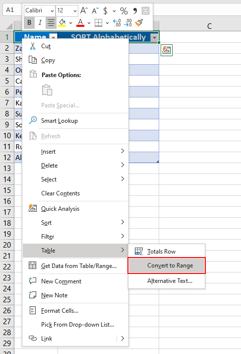
Now that the Table element is gone, we’re working with a regular range. The formula ahead will not result in a #SPILL! error and will also sort the names alphabetically:

Apart from the scenarios mentioned above, you might face the #SPILL! error in Excel if it runs out of memory. In that case, try using smaller ranges.

Hopefully, now you will be able to resolve the #SPILL! error in all the possible conditions. While you solve your #SPILL! errors, we’ll bring you some more tutorials to make sure your Excel rides are buttery-smooth.