Excel has its limits and it’s a good thing we’re not talking about temperament here. We'll name one limit and learn at length how to fix it. Excel has its way of showing large numbers and decimals. As it is, you won’t be able to make Excel display all the digits of the large number without pulling out some stops.
What we mean by a large number is a regular number over 11 digits and a decimal over 7 digits. What could these many digited numbers be used for? The number can be representing a debit/credit card number, phone number, or a numeric code. That makes it important for all the digits to be present, right?
Shortly after, you will get the details on why Excel rounds numbers. We will fix the problem of rounding decimals by increasing column width and setting the decimal places to an increased number. The fixes for rounding regular numbers will be through changing the cell format or converting the number to text. First, let's get an idea of what's going on.

Why does Excel Round Off Numbers?
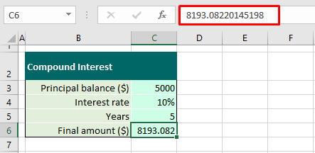
Before we start troubleshooting, we need to see what we’re dealing with. Excel takes a reasonably space-efficient approach to displaying numbers. A cell would generally display 8 digits in the default font and the General Number Format (also default). Decimals will also be displayed with 8 characters including the decimal point.
How numbers will be displayed depends on how many digits the number has. As mentioned, 8 digits would make a perfect fit with the default column size. For a 9-digit to 11-digit number that is entered (not pasted), the column will automatically increase its width to accommodate the number to a fit.
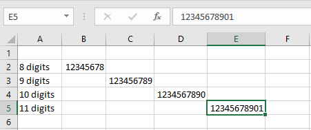
Column B contains an 8-digit number with unchanged width. As for columns C, D, and E, the column width has expanded to fit the added digits. But by adding the 12th digit, after expanding to its maximum automatic capacity i.e. 84 pixels, the number will be displayed with scientific exponential notation:
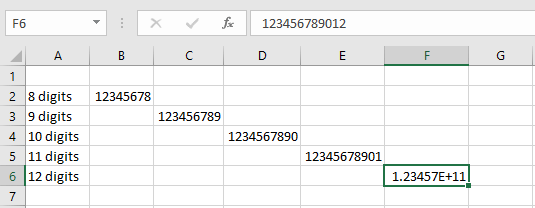
The 12-digit number itself can be seen in the Formula Bar while the cell displays the number in exponential notation.
From this we can gather that Excel rounds large numbers and decimals because of:
- The number is too large to be completely displayed other than in exponential notation.
- Insufficient column width.
- The format of the target cell
Note: The Excel treatment of numbers given above is with the assumptions that the Number Format is General, the font is Calibri size 11 by default and the column width has not been preset. In the case of preset column width, the width will not automatically expand for large numbers and will be shown in exponential notation.
Also, note that how much of a number is displayed doesn’t affect its actual value which can be seen in the Formula Bar.
We’ve explained the “what” and “why” part of Excel’s rounding of numbers. Now let’s go on to find “how” to counter the rounding to keep the numbers in their entirety.
Time to put a stop to the rounding!
Recommended Reading: Round Function In Excel
Method #1 – By Increasing Column Width
Increasing column width is the first way to fix Excel's rounding of numbers. This method works for decimals to a great extent and on regular numbers to a certain extent. With decimals, extending the column can display up to 10 digits of the number.
Considering what little numeric value a decimal has after the decimal point, a few digits displayed should be enough. But with certain calculations where decimals need to be multiplied by large numbers, you may want to see a few more digits after the decimal point.
A regular number will need extra column width for numbers with more than 9 digits. Up to 11 digits entered, the column width expands itself. Beyond that, expanding column width will be of no use as the numbers will still be displayed with exponential notation.
Either way, these are the steps you can use to increase the column width to stop Excel from rounding numbers:
- If the decimals are in multiple columns, to begin with, you need to select those entire columns. If the numbers are in one column, skip to the next step.
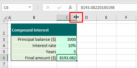
- Place the cursor at the column header border of the column containing the decimal.
- A double-pointed resizing arrow will appear.
- Double click when the resizing arrow appears or you can click and drag the column header border to a width of your preference.
Notes:
The column width can be increased before entering the numbers. All in all, it’s easier to see how much to increase the width after the numbers have been added.
If you’re faced with a stretch of hash symbols, that is also an indication that the column width needs to be increased. When the column is expanded, the hash symbols will clear and the number will be displayed.
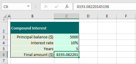
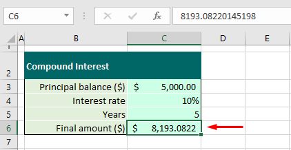
For our case, expanding the column has displayed 6 decimal places which are quite enough. However, if you must have the complete number shown in the cell, the decimal places can be increased by the buttons on the Ribbon.
Now you can increase the decimal places of a decimal to get all the digits to show but you can't apply the trick to a regular number, obviously. The way around that is to change the format of the cell and also applies to decimals. The details on this are right ahead.
Method #2 – Change the Cell Format
Changing the format of the cell to display numbers with more than 11 digits is a good trick to counter Excel’s rounding of numbers. You’ll find changing the cell format handy to show 11-digit to 15-digit numbers. Why do we need to use another tactic now? Increasing the column width will have no effect on numbers over 11 digits.
The default format of the cell in Excel is the General format. Changing this to specifically the Number format will open up the digits from the exponential notation and display them. You may choose to change the format before or after adding the numbers. Change the format of the cells with the following steps to stop Excel from rounding numbers. See the example below:
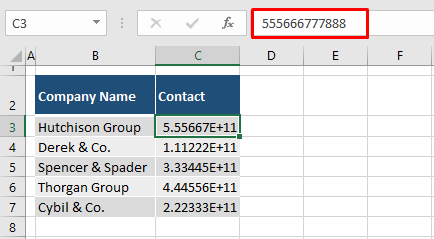
- Select the cells with the numbers.
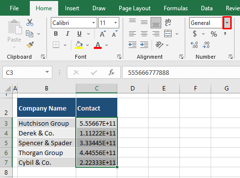
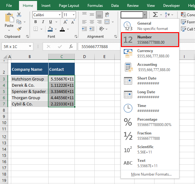
- In the Home tab’s Number group, click on the Number Format bar arrow and select the Number format from the list.
- A sample of each format is provided in the list. As in the list, the Number format will display the number with 2 decimal places:
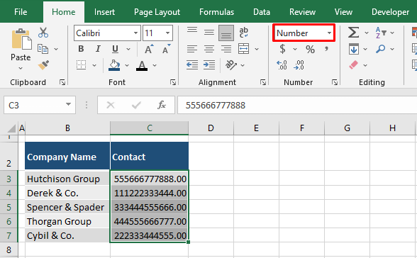
- In the Number Format bar, the format has been changed from General to Number. As a result, the selected numbers are displayed completely with 2 decimal places:
- To convert the numbers from decimals to integers, click on the Decrease Decimal button below the Number Format You will need to click twice to remove the 2 decimal places.
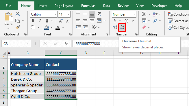
The decimals will be converted to integers:
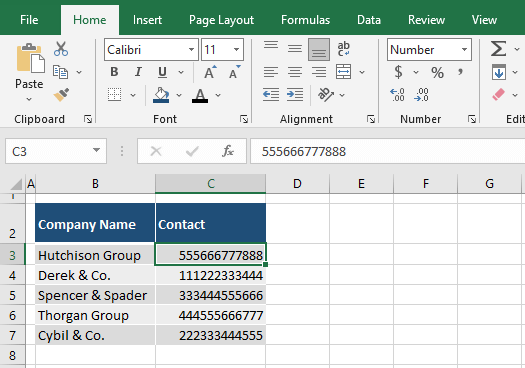
With that one tackled, let’s throw another spanner into the works. This trick will work for numbers under 16 digits. For any large number added to Excel (whether entered or via copy-paste), zeros will take place of the 16th digit onward. This is not just for display or as a format, the zeros will take place of the digits in the actual value. Like this:
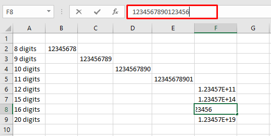
We have entered the 16th digit as the number 6 but it will be replaced with a 0:
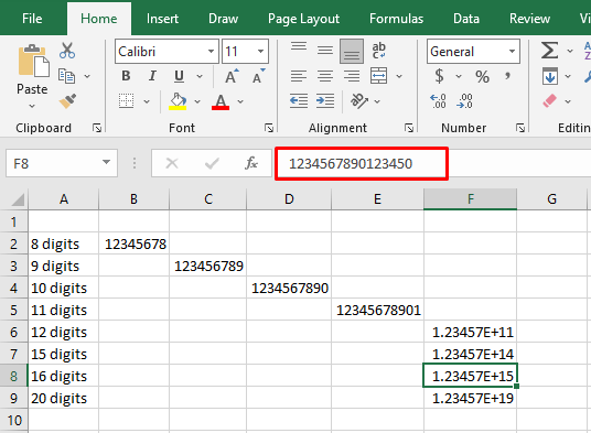
The same goes for any number that is from the 16th to the 21st digit; they will be stored as zeros:
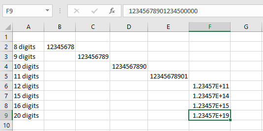
This replacement with zeros will also take place even if the format is changed to the Number format. So the way to deal with this is to not let the number be a number at all and change it to text. Find out all about it ahead.
Method #3 – Convert the Number to Text
This method deals with preventing Excel from rounding numbers with more than 15 digits. There are a few ways to do this. You can add a character or symbol to the number e.g. space character, hyphen, etc. especially if it is fitting for what the number represents (a space is added every 4 digits in a 16-digit card number).
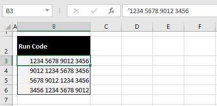
If you would rather not change the display of the numbers, one way is to add a leading apostrophe to the number. The apostrophe will change the number to text and will also not be displayed in the cell. All you need to do is add an apostrophe before adding the number:
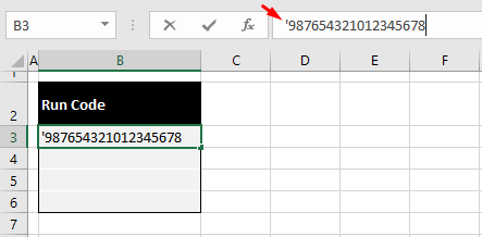
The numbers will be entered with the apostrophe in the value of the cell but will not be seen in the cell itself. There will also be an error notification icon when the cell with the number is in selection:
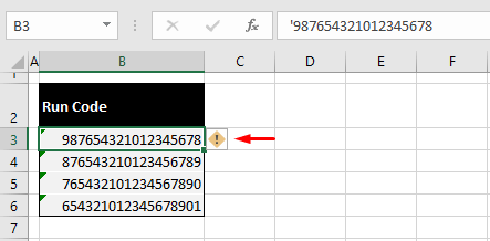
It’s no big deal removing these errors and we’ll show you what to do in a while. The issue with this method is the monotony and we find that the easiest way to contain large numbers exceeding 15 digits is to change the cell format to Text format.
Our preference for this method is because you can also copy-paste the numbers from another source after changing the cell format; you won’t have to enter each apostrophe and number. As easy as pie, this is how to change the cell format to Text:
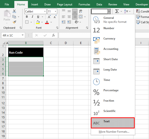
- Select the cells where the numbers are to be added.
- Use the Number Format bar in the Number group from the Home tab to select the Text
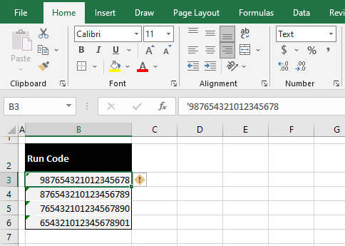
- With the cell format changed to Text, add the numbers to the formatted cells.
See what happened here? Adding a number to a Text formatted cell automatically adds a leading apostrophe. Isn’t that so much easier than doing it manually? Now for the errors:
- Select the range with the errors and click on the error notification icon.
- Select Ignore Error from the menu.
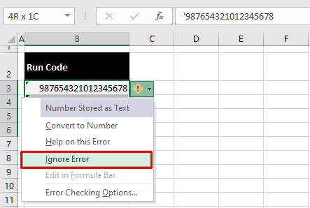
With the error removed, the numbers will be displayed with their whole value and will carry a leading apostrophe:
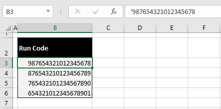
Note: Only apply this method if you’re dealing with numbers with 16 or more digits as the numbers, being in Text format, can’t be used in calculations or number functions.
Prevent Rounding Decimal Numbers/Currencies
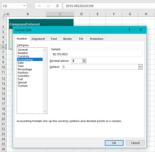
We have seen above, that decimals can be stopped from rounding by expanding the column and/or by changing the cell format to Number. That can be unfavorable if you want the Accounting or Currency Format. In that case, the number of decimal places can be set in the Format Cells dialog box so that the number isn’t rounded by Excel. Let’s do this with the example below:
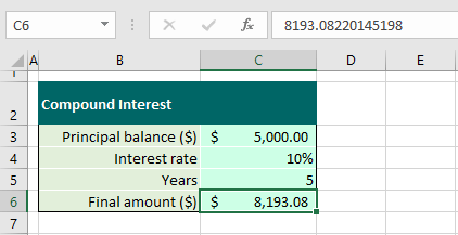
The number selected above is in the Accounting Format with 2 decimal places. As discussed earlier, with intricate calculations, it would make matters clearer to have more decimal places displayed. The following steps will achieve that:
- To open the Format Cells dialog box, right-click on the cell with the number and choose Format Cells from the context menu or press the Ctrl + 1
- The dialog box will open up in the format of the cell. Increase Decimal places from 2 to the number you want.
- Next, click on the OK command button.
The cell will show the number with the set number of decimal places:
Now that you’ve stopped Excel from rounding numbers, you can make a fair stop too. Rounding up this tutorial, we showed you how to keep a decent chunk of large numbers and decimals without Excel chipping them away. We’ll be back again to chip off more tricks while cracking this vast mystery called Excel. Do get back for your share!
 See what happened here? Adding a number to a Text formatted cell automatically adds a leading apostrophe. Isn’t that so much easier than doing it manually? Now for the errors: