How to Transpose Data in Excel (3 Quick & Easy Ways)

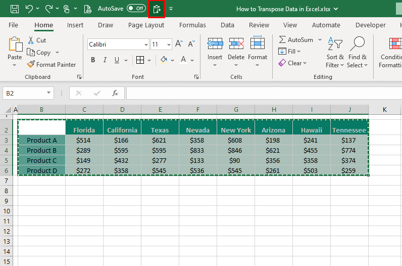
Transpose is an effectively powerful feature that switches the orientation of data quickly in Excel. Why would you want to change the data's orientation?

Going for more column-favored or row-favored data, opting to increase the data in height instead of width (or the other way round), compacting data, trying to improve readability or the visual for easier analysis. These are the top reasons for flipping the direction of data and transposing it.

Now what if we told you that this:

Is essentially the same as this:

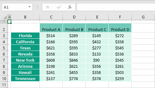
Isn't the latter easy on the eyes? What has happened here is that the column headers have been stacked as row headers and vice versa, taking the data layout along with it. All of row 1 goes as column 1, row 2 as column 2, and onwards and column 1 to row 1, and onwards. With row for row and column for column, the original data i.e. 5 x 9 becomes 9 x 5.

The switch is basically from horizontal to vertical and vertical to horizontal. Depending on your requirement, you may prefer one over the other and feel the need to switch things around. Literally. The transposed data takes up as many cells as the source data while switching the orientation.

So here's the scenario we're dealing with in the given example; the states are set as column headers and we need to merge more data to add more states to the dataset. As evident from above, adding more states will stretch the data's width. Since the products are only 4 with no intent to add to them soon, it would compact the data if the row headers were converted to column headers.

One way to compact data would be to change the alignment of the text in the column headers to 45 degrees but that's a functionality for another day. The option we're exploring today is how to transpose data in Excel and luckily, it's not something that you have to put too much effort into.

We've already shown you the transposed face of the data earlier. How to do that? Keep reading.

Get set transpose!

Method #1 – Using Paste Options

Transpose data in Excel using the Paste options from the right-click menu. This method is a copy-paste way of transposing data through one of the special options. Transpose through Paste options pastes the values along with the formatting.

Therefore, it is best to use this method of transposing data when you want the cells to retain their formats, to discard the original data, and when you don't want the figures linked between both the datasets i.e. the original and transposed datasets.

Once you've decided to use this functionality, you can follow these steps to transpose data in Excel using the Paste options:

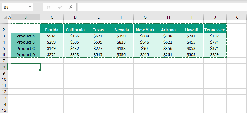
• Select the range of cells that you want to transpose.
• Press the Ctrl + C keys to copy the cells to the clipboard.
• 
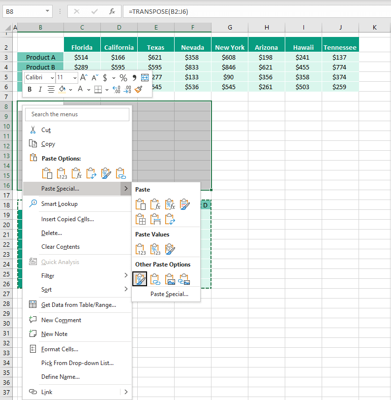
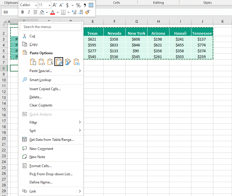
• Right-click on the new cell where you want to paste the transposed data (that is cell B8 for us in our case example) and choose Transpose from the Paste Options section in the context menu. The Paste Special submenu also contains the Transpose
• 
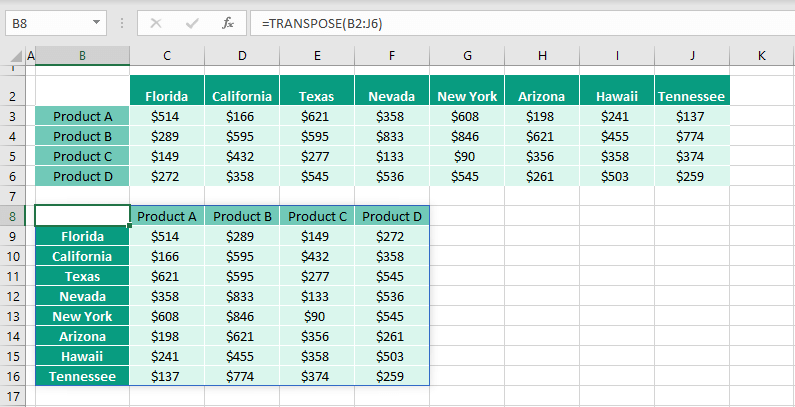
• The option will paste the transposed data in the new cell:

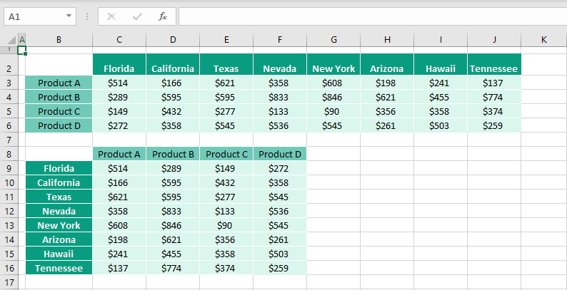
Since this method of transposing has no dynamic link between both datasets, you can delete the original set if it is not needed. Adjust any formats if required and voila:

Note: Be mindful of the location of the transposed data as the range required for the pasting should be free. The data won't be prohibited from pasting; it is so no data is overlapped, or important data overwritten accidentally.

Method #2 – Keyboard Shortcut

Use the keyboard shortcut given in this section to transpose data in Excel. This is the keyboard method of using Paste Special to apply the Transpose option. The keyboard shortcut to transpose data in Excel is:

Ctrl + Alt + V, E, Enter

The Ctrl + Alt + V keys open the Paste Special dialog box.

The E key marks the Transpose checkbox.

The Enter key selects the OK button.

The steps below will show you how to use the keyboard shortcut above to transpose data:

• Copy the dataset you want to transpose.
• Select the cell you are aiming to transpose the data to. We have selected B8 in our example case:
• 
• Now press the Ctrl + Alt + V keys together to access the Paste Special dialog box. Next, press the E key to check the Transpose And then when you hit the Enter key, the OK button will be selected.

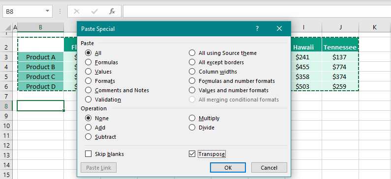
Once you hit the Enter key, the dialog box will close with the selection of the OK button and the selected dataset will be transposed to the chosen location:

Method #3 – Using TRANSPOSE Function

Data can be transposed in Excel with the TRANSPOSE function. The TRANSPOSE function converts a horizontal range of cells to a vertical range or vice versa. You only need to supply the range to the function and it will transpose the data in the range to the target cell, spilling the result. The formula is very simple and we are using the following one to transpose data using the TRANSPOSE function:

The target cell for the formula is the cell where you want to transpose the data which is B8 in our example case. Make sure the target location has enough cell space to accommodate the results of the transposed data. Start by entering the formula there. As for the array argument, this is the data you want to transpose and you can type it in or select it on the sheet using the mouse.

Now the second part of the function is to enter it. Since the TRANSPOSE function is used only in array formulas, the formula needs to be formed as such. If you are equipped with a Microsoft 365 subscription, all you need to do is hit the Enter key to confirm it as a dynamic array formula.

But for any other version of Excel, you will need to use the Ctrl + Shift + Enter keys instead of just the Enter key to enter it as a legacy array formula. The Ctrl + Shift + Enter keys enter the formula enclosed in curly braces. Thus, the formula becomes:

Below you can view the output of the TRANSPOSE function applied to our case example, the results are spilled from the formula cell taking up as many cells as the original data to transpose it:

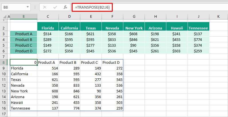
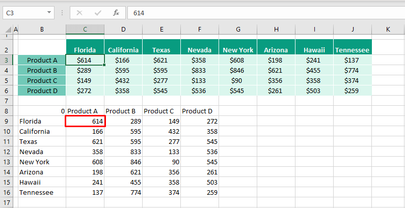
You might have noticed the absence of formatting but check out the perk of using the TRANSPOSE function. Any change that we make to the source data gets reflected in the transposed data. We have changed the first sales figure from 514 to 614 in the example and the transposed data has responded with a match:

Notes:

Since the original data is the range fed into the formula, you cannot delete it as done using the Paste option. The TRANSPOSE function forms a one-way link between the two datasets; the values can only be changed in the original dataset.

Since the transposed data is the spilled result of the function, changing a value in the transposed dataset will result in a #SPILL! error in the formula cell as the spill range will be barricaded by the entered value.

If you still so wish to make a change in the transposed data, you can paste the values of the data back on itself. This will sever the connection between the datasets in which case, it's a better idea to use the Paste option instead of the TRANSPOSE function.

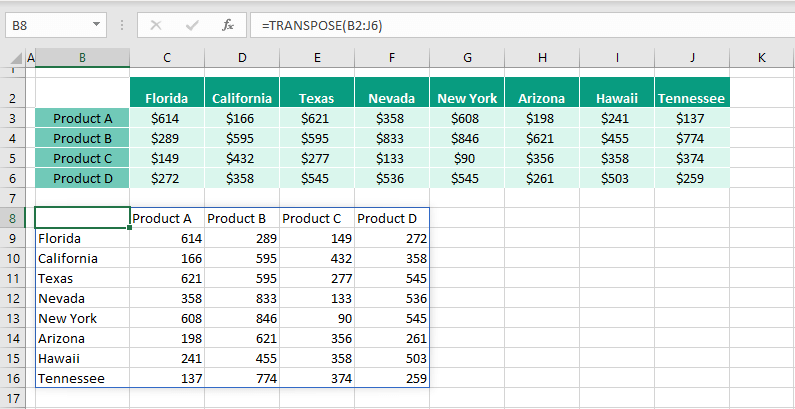
In our case example, the first cell is blank which has been transposed as 0 as the TRANSPOSE function only results in the values of the dataset. You can hide the 0 by changing the font color to the cell's fill color (white in this case). We have changed B8's font color to white:

As you may have noted, the TRANSPOSE function only transfers the values of the source data and not the formatting. In case you want the formatting along with the dynamic linked data, you can copy just the formats from the original dataset. If that's too much hassle, here's a little trick. You can transpose the data again to another location with the Paste option.

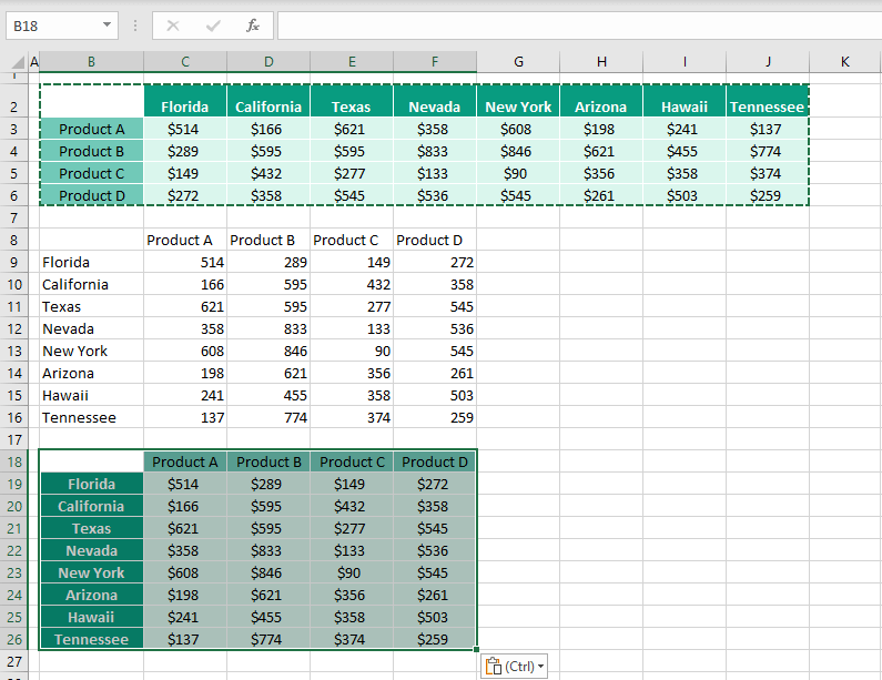
Since the Paste option also copies the format, copy this data, paste just the format to the TRANSPOSE function results:

Then you can delete the Paste option dataset. Now you have the transposed data with the dynamic link from the TRANSPOSE function and the formatting rendered from the Paste option. Best of both worlds.

Paste Option vs TRANSPOSE Function

In terms of the values involved, both methods change nothing in the values and transpose them as they are, covering the same range orientation.

The immediate visual difference that you can notice is that the Paste option copies the formatting and the values of the original dataset while the TRANSPOSE function only transposes the values. But the core distinction between the two options is that the Paste option gives a static result while the TRANSPOSE function gives a one-way dynamic result that is linked to the source data.

And we have already learned from the trick above that if the formatting is so crucial, it can always be taken from the Paste option result and applied to the TRANSPOSE function result.

The transposed data using the Paste option can be edited as it is pasted values. Editing transposed data produced from the TRANSPOSE function is not possible as it would result in a #SPILL! error. With the function, blank cells (including the blank cell of a merged cell) are transposed as 0. The Paste option pastes blank cells and merged cells as they are.

The original dataset can be deleted in the Paste option since it is not linked to the transposed data but with the TRANSPOSE function, the original dataset needs to remain since its range is fed into the function to return the results. The TRANSPOSE function can transpose the data from a Table, the Paste option cannot and requires the Table to be converted to a range first.

Therefore, the matters to consider for picking the method for transposing data involve a dynamic link to the data source, editing the transposed data, keeping the original dataset, and formatting.

Add Transpose Option to Quick Access Toolbar

If data transposition is something you do often, you might find the option to do so in the Quick Access Toolbar handy. The Transpose command is a quick way of applying the Paste option with a single click. The details to add the Transpose option to the Quick Access Toolbar and then use that option are given below:

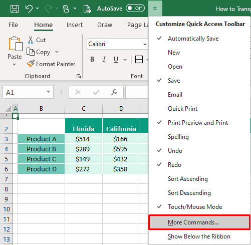
• Click on the Customize Quick Access Toolbar button in the title bar and choose More Commands from the drop menu.
• 
• You will be redirected to the Quick Access Toolbar tab in Excel Options.
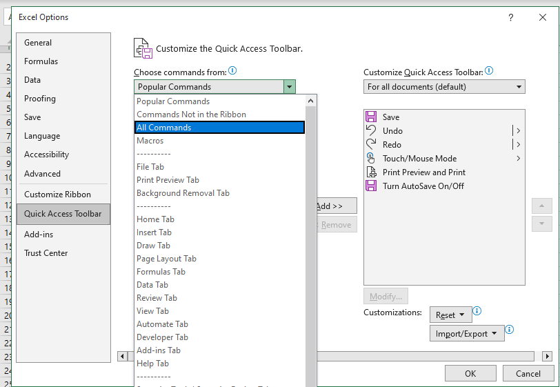
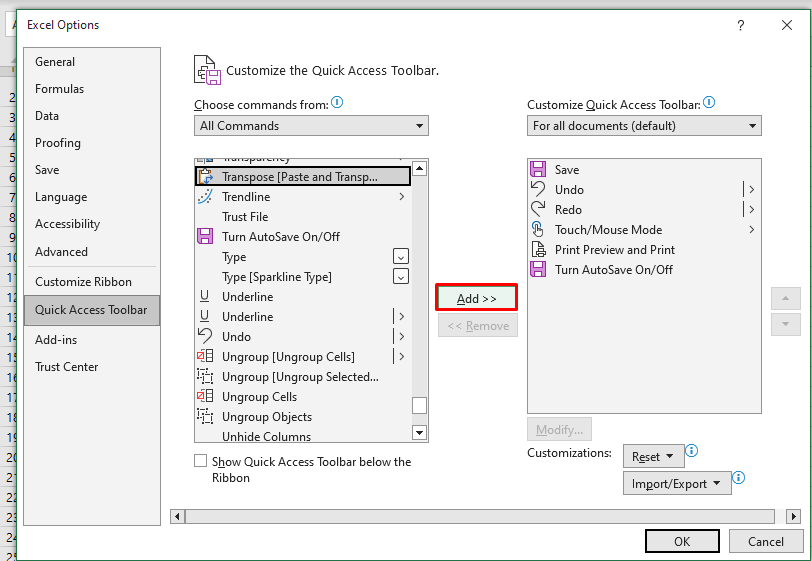
• Click on the drop arrow of the Choose commands from bar reading Popular Commands. Select All Commands from the list to display all the commands.
• 
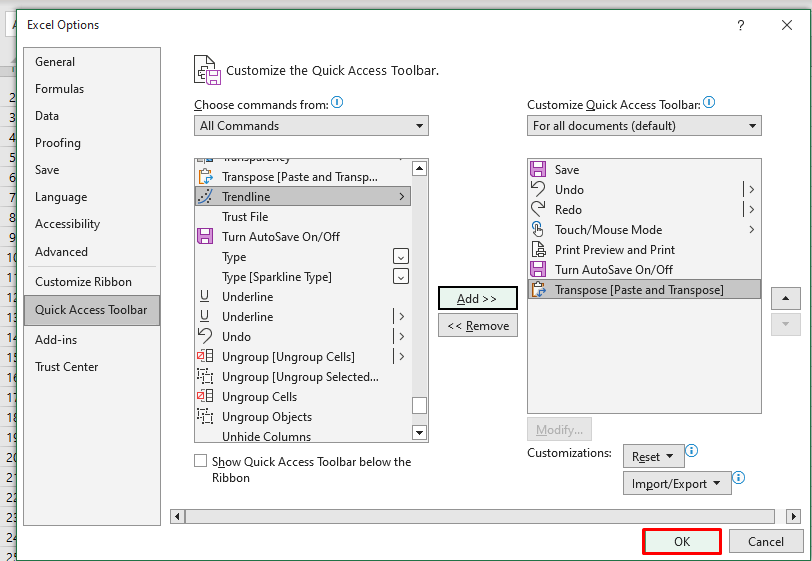
• The commands are in alphabetical order so scroll to the T section or type "transpose" and it will lead you to the command. Select the Transpose [Paste and Transpose] command and click on the Add button to add the command to the Quick Access Toolbar.
• 
• Once added, hit the OK button to confirm the setting, close the dialog box and return to the worksheet.
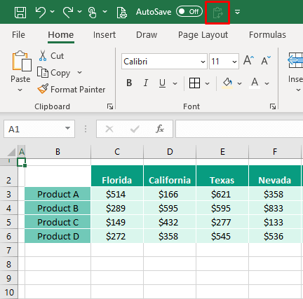
• The Transpose command will be added in the Quick Access Toolbar:Currently, it will be disabled but is activated as soon as a cell is copied.To use the Transpose command to transpose data:
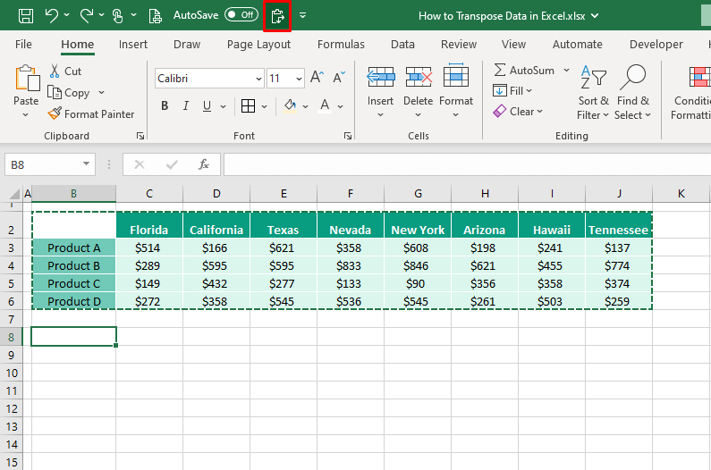
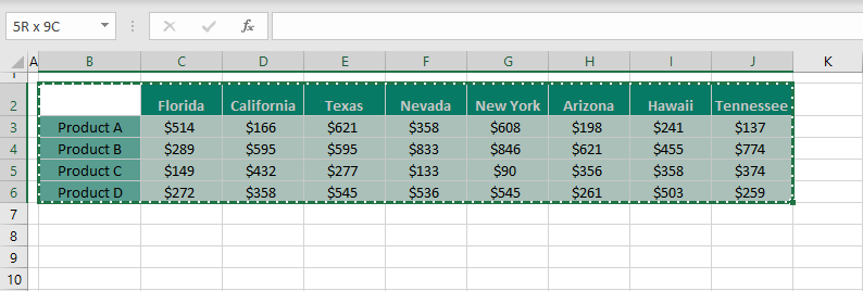
• Copy the data. The Transpose command is now enabled:
• 
• Select the cell (as we have selected B8) that is to be the starting point for the transposed data.
• Click on the Paste and Transpose command in the Quick Access Toolbar.

As quickly as the toolbar promises, the data will be transposed to the selected location:

You may be new to transposing data but with this tutorial, hopefully you aren't new to how to get it done in Excel. Think about what you want from the transposed material before selecting a method. We'll supply you with more Excel brain fodder soon enough. Race you to the top? Ready? Tricky? Go!