Excel COLUMN Function – How To Use

The COLUMN function returns the column number of a specified cell reference or range of cells. For a range of cells, the COLUMN function will spill the results, returning the column number of each cell in the given consecutive range. The function is very useful when dealing with large datasets where the users can identify column numbers quickly.

It is important to note that the COLUMN function returns the column number relative to the first column in the worksheet. Cells in Column A will be 1, Column B will be 2, and so on.

Syntax

The syntax of the COLUMN function is as follows.

Arguments:

The COLUMN function accepts only one argument.

'reference ' – It is an optional argument that contains the cell or range of cells for which we need the column number. It is worth noting that the reference argument cannot include multiple cell references.

Important Characteristics of the COLUMN Function

Some noteworthy features of the COLUMN function are as follows.

• If the argument reference is omitted, the COLUMN function returns the column number of the cell in which it is used. The column number of the cell that contains the formula is returned.
• If the at symbol (@) is added at the beginning of the COLUMN function, it ignores the array input and only considers it a single value which is the first value of the array. It is called an implicit intersection operator.

Examples of COLUMN Function

The COLUMN function comes in very handy when dealing with large data and is used for data analysis. Let's explore various applications of the said function with the below-mentioned examples.

Example 1 – Simple Use of COLUMN Function

Here we have taken different input values for the reference argument to learn how the COLUMN function behaves with them.

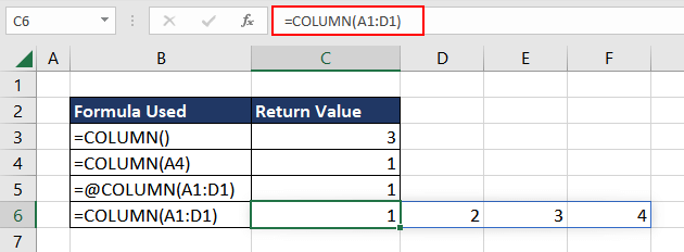
In the first example, as the argument is left empty, the function returns the column number of the cell containing the formula which is C3, and hence the resulting column number 3. In the next example, the formula returns the column number of cell A4 which is 1.

The next two examples show different ways to use cell range as an input value for the reference argument. In the third example, even though the input value of the COLUMN function is a cell range, the formula returns the column number of only the first cell which is A1, hence the return value of 1. This is due to the use of an implicit intersection operator as mentioned above.

In the last example, the COLUMN function returns the column number of each value in the cell range A1:D1 which is 1,2,3,4.

Now that the basic use of the COLUMN function is clear, let's move on to some more examples of the function.

Example 2 – Locating Last column in Range

Suppose we have a data table that lists sales data for different products across different months, with each row representing a product and each column representing a month.

Now we wish to create a chart that shows the total sales for each month but to do this, we need to find the last column in the table so that we can select the data range for the chart.

We can use a combination of the COLUMN and COLUMNS functions to find the rightmost column in any range. We will first find the smallest column number in the given cell range. Then we will add the total number of columns and subtract 1 to account for the fact that we want the last column, not the total number of columns.

To find the smallest column number, the formula used will be

The COLUMN(B2:H7) will return the array {2,3,4,5,6,7,8} and the MIN function will return the smallest value in this array, which is 2 in this case. Adding the total number of columns, the updated formula will be as follows.

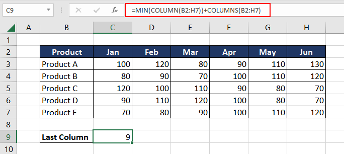
Now, the final step is to subtract 1. The reason we subtract 1 is that the smallest value represents the first column in the range, so adding the number of columns would give us the column number of the last column + 1. The final formula used will be as follows.

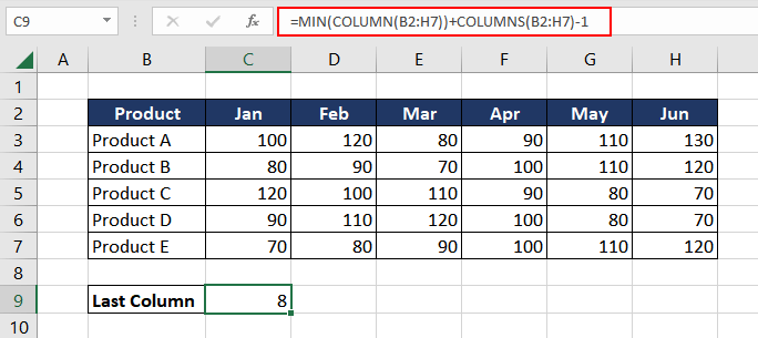
Example 3 – Adding a Value on Every 3rd Position

In this example, we have a dataset that shows a fixed income of 2500 USD every month for a year. Now, every 3rd month, we wish to enter an additional income of 1200 USD which we get from the selling of shares.

To automate this, we will use the COLUMN function and check if it's a multiple of 3 as we wish to add a value in every 3rd column. If it is a multiple of 3, we add 1200 USD as an additional income or we add 0. We will use a combination of MOD and COLUMN functions to get the desired result. The formula used will be as follows.

The COLUMN function returns the column number of cell C2 which is the third column and hence the value will be 3. Wrapping it in the MOD function, the formula takes the column number of C2 and divides it by 3, returning the remainder. In this case, 3 divided by 3 is 1 with no remainder.

As the formula is dragged or copied horizontally to adjacent cells, the COLUMN function's return value increments by 1 for each cell. This is what creates the pattern for every 3rd cell. Now, we use the basic IF function using the below-mentioned logic.

If the return value from the MOD function is 0, then return 1200, otherwise, return 0. The formula used will be as follows.

Using a similar logic, we can create automation for every nth value by making a few adjustments to the formula.

Example 4 – Finding Sum of Nth Column Value

Suppose we have a dataset of everyday sales for different products. To analyze the performance of the products over time, we need to calculate the total sales for each product on specific days.

Depending on the requirement, we will try to curate a formula to find the sum of every nth value where n represents the day. For example, if we want to find the total sales for every second day, we can use the formula to calculate this value.

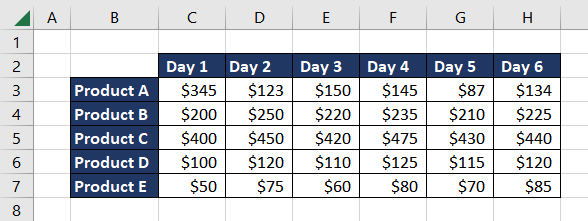
We will first calculate the column number of the leftmost cell and ensure that it is to be considered 1. The formula used will be as follows.

The formula COLUMN(C3:I3) returns an array of column numbers corresponding to each cell which will be {3,4,5,6,7,8,9}. We will then subtract the first column number from each column number in the array which will be 3 in this case. The resulting array would be {0,1,2,3,4,5,6}

Lastly, we will add 1 to each value to ensure that the column number of the leftmost cell in the range is considered column 1, not column 0.

This is an excellent way to ensure that Excel considers the leftmost column of your dataset to be the first column irrespective of its placement in the worksheet.

In the next step, we will use the MOD function to determine whether the column being evaluated is the nth column (Column I). When the column number is divided by the value of n, the MOD function will return the remainder value. If the return value is 0, we have found our nth column. The formula used will be as follows.

Now we will simply check and filter if the return value of the MOD function is equal to 0. The formula used will be as follows.

As the last step, we will use a double negative operator (–) to convert the TRUEs and FALSEs to 1s and 0s. We will then use the SUMPRODUCT function with the resulting array of 1s and 0s and the range of cells being evaluated (C3:I3 in this case), which will give us the sum of the nth column for that particular row. The final formula used will be as follows.

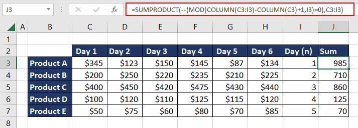
All the days of Product A sales have been summed as 985 based on the value of n as 1. Every 2nd value for Product B and every 3rd for Product C (and so on) is summed as per the n values in column I. This will allow us to gain valuable insights into the performance of each product and identify any trends or patterns that may exist over time.

COLUMN Function VS COLUMNS Function

Now we already know that the COLUMN function is used to return the column number of a cell reference. It accepts a cell reference as an argument and gives the reference's column number.

For example, if you have a value in cell B3, then using COLUMN function, would return the value 2, which represents the column number of cell B3.

On the other hand, the COLUMNS function returns the total number of columns in an array or range of cells. It takes an array or range of cells as its argument and returns the number of columns in that range.

For example, if you have a range of cells A1:C3, using COLUMNS function on the range would return the value 3, which represents the number of columns in the range.

It is important to understand the difference between the COLUMN function and the COLUMNS function, as they have similar names but serve different purposes in Excel. Confusing these two functions could lead to errors in your calculations or data analysis.

Practice the COLUMN function and leverage its capabilities for data analysis. It can save time and effort while working with large and complex data and will improve productivity and efficiency. We will soon be back with another exciting Excel function.