Excel CHAR Function – How To Use

CHAR function, also known as the character function, is one of Excel's text/string functions. It accepts an ASCII value as an input and returns the character corresponding to that ASCII value. Each number that is entered into the CHAR function has an individual character allocated to it.

The term "ASCII" refers to the American Standard Code for Information Interchange, where each bit stands for a different character. Numbers, alphabets, punctuation, special characters, and non-printing characters are all included in ASCII.

CHAR function is very useful when we wish to type a character not available on our keyboard or use a character that is also used as a wildcard character. A wildcard is a symbol that can be used in place of one or more characters to represent them.

Syntax

The syntax of the CHAR function is as follows:

Arguments:

'number' – is a required argument. It is an ASCII number ranging from 1 to 255, corresponding to a character.

Important Characteristics of the CHAR function

One of the most important features of the CHAR function is that the character code varies with the operating system. Windows OS works on ANSI/ASCII character set, whereas MAC/ Apple OS uses the Macintosh character set. Therefore, the same input number argument will give different results on different OS.

Other notable characteristics are as follows:

• The output of the CHAR function is always a text value.
• If the input argument number is out of the range (less than 1 or more than 255), Excel returns a #VALUE! error.
• The argument number also does not accept a non-numeric value and results in a #VALUE! error.

Examples of CHAR Function

CHAR function is usually used in sync with other Excel functions to bring out the required results. When used directly, it simply returns the corresponding character to the input number, as seen in the example below.

Column B contains the value of the input argument – number, and column C contains the following formula with the CHAR function:

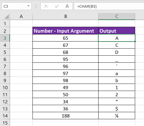
It is worth noting here that the distance between the upper and lowercase characters is exactly 32 numbers. The number for a lowercase "a" is 97, which is obtained by adding 32 to 65; the number for an uppercase "A.".

Example 1: Mailing Address using Line Break

One of the most talked about CHAR functions is a line break. In Excel, placing a new line within a cell is known as a line break. We can quickly move to the next cell using the "Enter" key but to move to a new line within a cell; we must add a line break inside a cell using the CHAR function. But a line break is as easy as pressing the Alt + Enter keys, right? Not when you have plenty of them to add.

Depending on whether we are using Excel on a Mac or Windows OS, a different character is used for a line break. CHAR(10) for Windows and CHAR(13) for Mac. Here, we will explain using the Windows version – CHAR(10).

Suppose we have the guest list, which contains their name, address, city, county, state, and zip code (as seen in columns A to F). We wish to compile all of them and finalize the mailing address list for the invitations. Doing it manually would take a lot of time, but we can use the CHAR function and do it in minutes.

To combine the data from all the columns to form the mailing address, all we need to do is add a line break after each cell data. That means the formula should go as: Name (line break) Address (line break) City (line break) County (line break) State (line break) Zip.

The final result (mailing address) should look like this, pretty neat, right?

Now, let's put it in the form that Excel understands. As we will be using multiple functions and text in one formula, we must join them or concatenate them using one of the concatenation functions or ampersand (&). The CONCATENATE function or CONCAT function joins different text strings (containing numbers, strings, values, or functions) into one string. Therefore, the final formula to be used is:

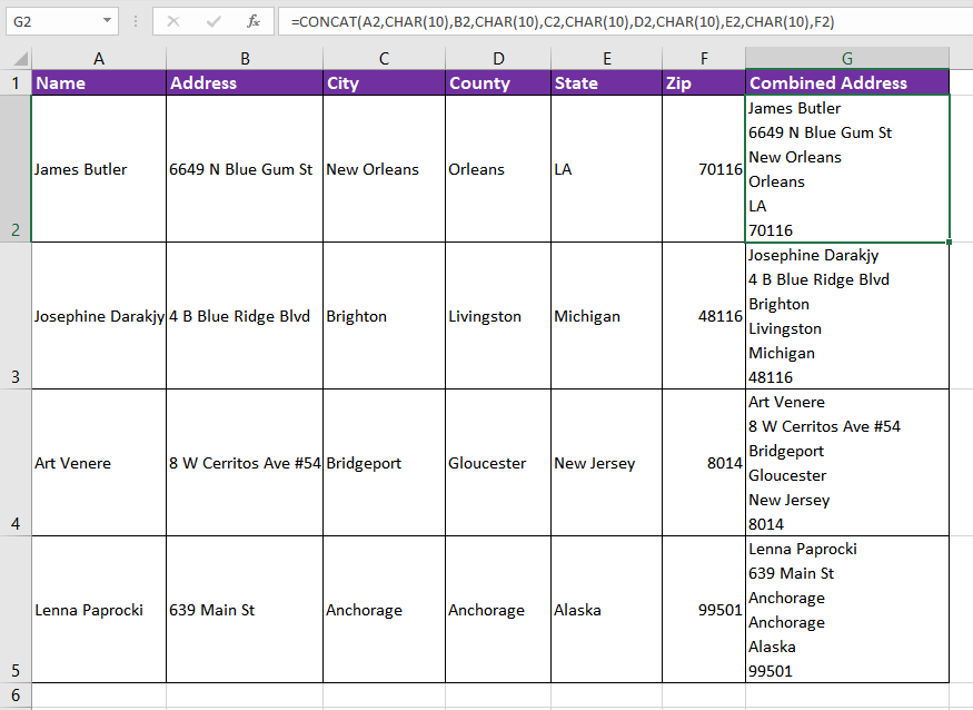
Alternatively, we can use an ampersand (&) in the formula.

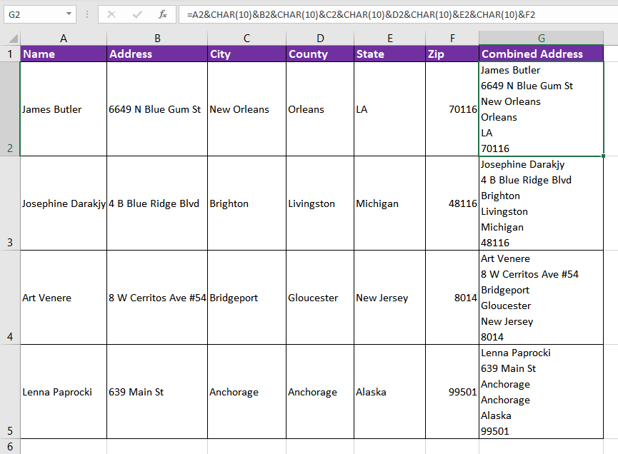
 Note: Instead of adjusting the row and column width to make the data look presentable, use the Wrap Text functionality of Excel. After entering the formula, the cell might look like this:

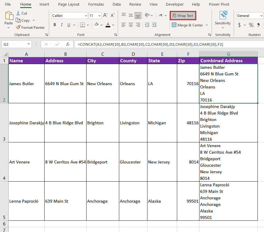
With the Wrap Text feature, all data in a cell is displayed, even if it extends beyond the cell's edge. To make it look more orderly, Select the cell and click the Wrap Text button under the Alignment group on the Home tab.

Example 2: Creating Email IDs of New Employees

In this instance, say you are the hiring manager, and each time a new employee is hired, you are responsible for creating their work email IDs. Rather than doing it manually, why not use the CHAR function and automate the process?

The email ID includes the first two characters of the employee's first name, the first two characters of the last name followed by at sign (@), and the company's domain name. For Example – If the latest employee's name is Mark Waycott – his work email ID shall be – [email protected].

Column B contains the employees' first names, and column C contains the last names.

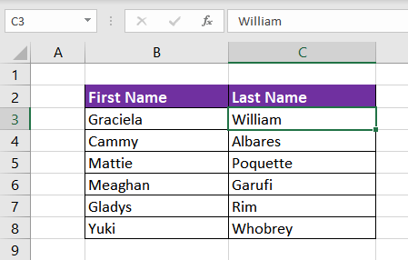
Now, let's compile (concatenate) the email IDs using the CHAR Function. As we need the first two characters from the first & last name, we will use the LEFT function. The LEFT function extracts the given number of characters from the string starting from left to right. So, our email will be as follows:

In Excel, we will use it as follows:

The first name is in cell B3. Extract the first 2 characters of the first name using the LEFT function – LEFT(B3,2). Then, extract the first 2 characters of the last name – LEFT(C3,2). Now, using the CHAR function for (@), which is CHAR(64), and lastly, adding the company domain name as text in double quotes ("").

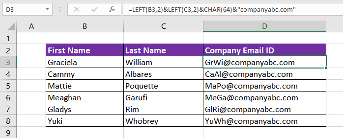
We will get our email ID in cell D3. But, as we know, the email IDs are always in lowercase. So, let's wrap everything in the LOWER function of Excel to convert our email addresses into lowercase letters. The final function to be used is as follows:

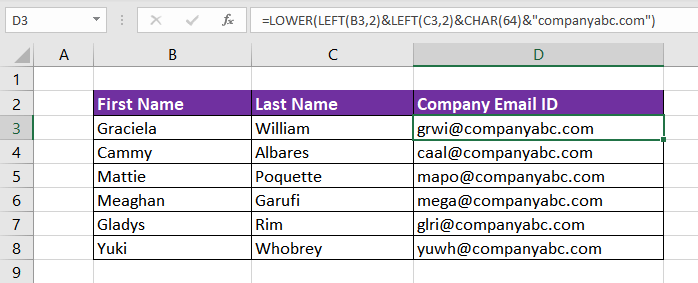
Example 3: Double Quotes in a Formula

Using double quotes in a formula in Excel can be tricky as, by default, double quotes ("") are used to signal the beginning and end of a text/string argument in a function. So, suppose we wish to print- The Marvel Movie "Iron Man" is a must watch. on Excel where the movie name is input from another cell. We will have to use additional double quotes as escape characters in that case.

Escaping a character means we direct Excel to regard a special character as literal text. In this case, double quotes must be regarded as text. So, the formula used will be:

To make this easier to understand, let's space the double quotes out, so you know which argument they belong to.

Now you can see that &B3& is surrounded by two pairs of double quotes instead of three. One pair of double quotes has The Marvel Movie enclosed in it, and one pair encloses is a must watch. The outer double quotes of &B3& encloses all the inner text and contents of the cell reference as text. This means that the text in B3 i.e. Avengers: Endgame and the inner double-quotes surrounding &B3&, both will be treated as text.

Using double quotes in formulas can be misleading as they can also be used to denote an empty text string ("" denotes empty text). Moreover, too many double quotes seem confusing and inelegant. We can instead use the CHAR function with the code value 34. CHAR(34) will return double quotes.

So, simply replacing the inner double quotes with CHAR(34) and keeping the outer double quotes so the inner value is taken as text, the final formula would be as follows:

We will get the same result in a much more elegant manner. That's how useful the CHAR function is.

Example 4: Remove Unwanted Character

In the following example, we received the price list of flowers we requested for an upcoming celebration. After downloading, we tried to add the price of all the flowers but could not due to the dollar sign ($) added to each price.

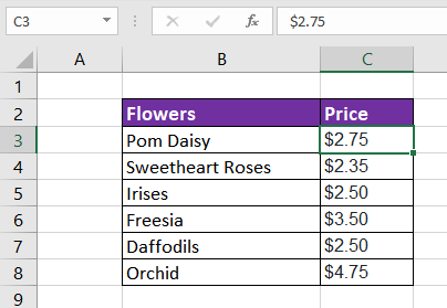
Removing the dollar sign from each price in column C manually would take a lot of time and effort. Instead, we can use the CHAR function to remove it. The ASCII code for the dollar sign is 36.

We will use the SUBSTITUTE function along with the CHAR function. Excel's SUBSTITUTE function is very useful to replace or substitute a given text with another text in a cell. In this case, we will substitute the dollar sign with an empty string. So, the final formula would be as follows:

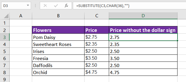
Example 5: Removing different characters from a single string

Assume that we downloaded some book titles from the internet to use further. When we downloaded them, we noticed some special characters in between the string. We obviously cannot copy them like this, so use the CHAR function logic as shown in the previous example to remove all the unwanted characters.

Column B contains the downloaded data. As we can see, there are three different types of characters in the string, unlike the previous example where there was just a dollar sign.

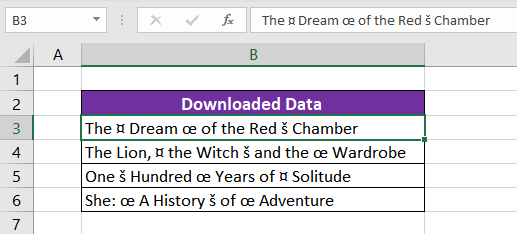
Before we compile the final formula using CHAR and SUBSTITUTE functions, note that these are the ASCII codes for the characters in the downloaded data.

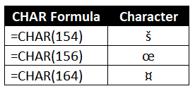
Now, removing the first character (š), the formula used will be

Now, we can use the partially cleaned string as an input string for the next substitute function to remove the remaining two characters. That means we will use a nested SUBSTITUTE function. So, by removing the next character (œ), the nested formula will be

Similarly, removing the last character (¤), the final formula will be as follows:

The character removal has left a leading and trailing space enclosing it. To give it a finishing touch, remove all the extra spaces, except a single space between words, using the TRIM function. Wrap the final CHAR & SUBSTITUTE function in the TRIM function to get the desired result.

CHAR vs CODE Function

Now that we have fully understood the meaning and application of the CHAR function, we must also have a brief idea about the reverse of the CHAR function. What if we don't know the corresponding value of a character?

We can easily use the CODE function. The CODE function is the reverse of the CHAR function. It accepts the character as the text argument and returns its corresponding number or code.

For example following formula returns '%'.

Now, if you try to find the char code of '%', you can use the following formula:

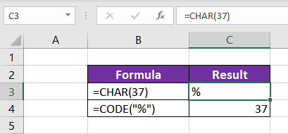
Pretty easy, right?

Alright, with this, we've covered the CHAR function inside out. Consider yourself an expert on the CHAR function once you've practiced these formulas thoroughly. While you keep yourself busy with the CHAR function, we'll have another Excel function loaded up, ready to fire away!