Excel DOLLAR Function – How To Use

The DOLLAR function is categorized as a text function in Excel. It converts a number to text but in currency format. The currency symbol and format depend on the computer's local language setting.

The DOLLAR function also comes with out-of-box rounding capabilities.

Syntax

The syntax of the DOLLAR function is as follows:

Arguments:

The DOLLAR function accepts two arguments, and details of each are given below:

'number' – This is a required argument that accepts the input value that is to be converted. The number argument can be a direct value or a cell reference containing the data.
'decimals' – This is an optional argument. The decimals argument indicates the number of digits to the right of the decimal point. If left blank, the default value is taken as 2. If the argument is negative, the function rounds the mentioned number of digits left of the decimal point.

Important Characteristics of the DOLLAR function

One of the most important characteristics of the DOLLAR function is that it converts the input value to a text format, so further numeric calculations with the final output are not possible but can be used as a text value. Other features of the DOLLAR function are as follows.

• The currency sign and format used by the DOLLAR function are picked up automatically as per the computer's regional settings. One can always change it as per their requirement.
• If the value in the number argument is non-numeric, the DOLLAR function returns a #VALUE! or #NAME? error.
• When the value of the number argument is negative, the DOLLAR function removes the minus (-) sign and adds parenthesis to the return value (like the Accounting format).
• When the value of the decimals argument is negative, the number will be rounded to the left of the decimal point.
• When the value of the decimals argument is negative and is greater than the number of digits before the decimal point in number, the DOLLAR function returns 0.
• The decimal places of the return value are to be defined in the function since the Increase and Decrease Decimal buttons in the Home tab cannot be used on the return values.

Examples of DOLLAR Function

As the DOLLAR function rounds off a number depending on the decimals argument, let's understand how the function behaves with different input arguments.

Example 1 – Plain Vanilla Formula for the DOLLAR Function

We have already learned that the DOLLAR function accepts two arguments. So, in this example, we take different values of both the arguments in columns B and C.

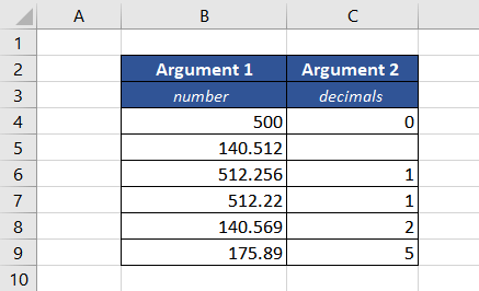
We have tried to cover all possibilities to better understand the DOLLAR function. The formula used will be as follows.

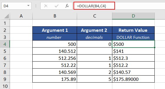
Now, let's understand the return values in all the different scenarios.

The first case is straightforward, whereas in the second case, the value of decimals is null. So the function rounds it off to zero places. As the number after the decimal point is equal to 5, the number is rounded up and the final value is 141.

If the decimals argument is greater than the number of digits after the decimal point, the DOLLAR function adds as many trailing 0s as required to achieve the input argument. This is seen in the B9, where the required decimals value is 5.

Example 1.1 – Using Negative Value in Argument

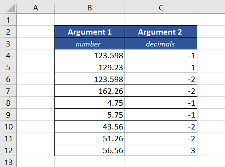
In the next few cases, the value of the decimals argument is negative, which translates to the position on the left of the decimal point.

We have taken a similar dataset as above containing the input values of both the arguments of the function in columns B and C.

The formula used would be the same as above.

Following are the return values for different input arguments.

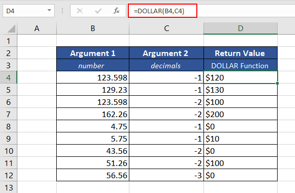
In the case of a negative decimals argument, It will round up or round down to the nearest 10s, 100s, and so on, depending on the value in the decimals argument. Let's understand it further with the example.

In the first case, the decimals argument value is -1, so the number checked will be on the ones place to the left of the decimal point, which in this case is 3. As it is less than 5, the number will be rounded down to the nearest 10, which is $120.

In the next case, the DOLLAR function rounds up to the nearest ten as the number on the first position to the left is more than 5, resulting in $130.

Moving on, if the decimals argument is -2, as in the case of values in cells B6 and B7, we will check the tens digit on the left of the decimal point. In cell B6, the input value is 123.598, so the tens digit is 2; hence, the DOLLAR function will round it down to the nearest 100, which is $100. Similarly, for B7, since the tens place digit is 6, the number is rounded up to $200.

The same is the case for values in cells B8 and B9. As the decimals argument is -1, we check the ones digit which is less than 5 in B8 and equal to 5 in B9. So, rounding it off to the nearest 10 gives us 0 in the case of B8 and 10 in the case of B9.

The last example is one of the characteristics of the DOLLAR function, which is if the absolute value of the decimals argument (in case of a negative number) is more than the number of digits before the decimal point, the return value is 0.

Hopefully, now you have understood how the DOLLAR function works when supplied with a negative value in the decimals argument.

Example 2 – Using DOLLAR Function with Concatenation Operator

In this example, we have received Facebook's stock price for 10 days. Now we wish to concatenate the stock price with the text for email purposes and make a sentence out of it.

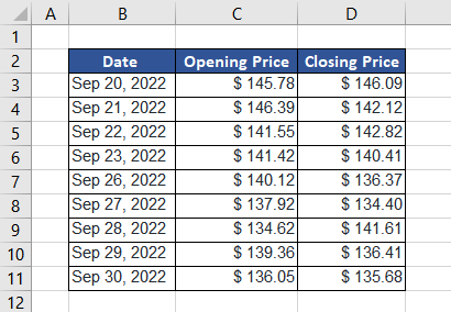
We tried to directly use the concatenation (&) with text using the following formula.

The return result is as follows.

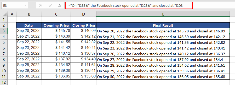
As observed in column E, the sentence form loses the currency formatting of the stock prices carrying just the numeric value. It is not ideal as it might be confusing for international users. Since currency formatting is lost during concatenation, one application of the DOLLAR function is to concatenate the number with the currency value to a text string using the said function.

As the default value of the second argument is 2, we will only insert the first argument in the DOLLAR function. The formula used will be as:

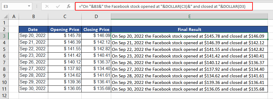
Now, the sentences in column E can be directly sent in emails. We can also use this application of the DOLLAR function while forming sentences with currency exchange rates, fuel prices, or prices of the products from your business.

Example 3 – Calculating Within the DOLLAR Function

Suppose you own a stationery business and have received a few customer orders. Now, you wish to quickly calculate the total amount payable by each customer and directly create their mail messages.

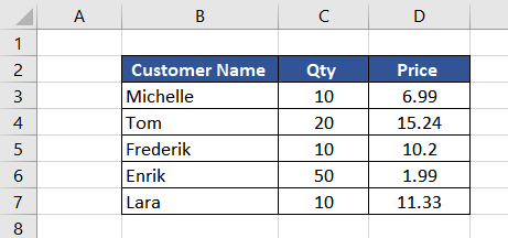
One way is to calculate each total and then mail them separately.

We can use the DOLLAR function to reduce the number of steps, as it allows in-function calculations. That way, the final value would be in currency text format and can be clubbed with other text.

The formula used will be as follows.

The above formula, if decoded, will translate to the following logic.

The text we wish to write is combined with the customer's name from column B. This is then combined with the DOLLAR function, where we directly calculate the total amount by simply multiplying the quantity and the price. The DOLLAR function first computes the calculations and then converts the value into currency text format.

Now that the entire return value is in text format, we can directly mail our customers.

DOLLAR Function vs. TEXT Function

We have already understood that the DOLLAR function alters the format from number to text using the currency format. The TEXT function also converts a numerical value into text but is a more exhaustive and versatile function than the DOLLAR function. In a way, the DOLLAR function is a subset of the TEXT function.

The TEXT function can be used to convert all kinds of values into text format in the given number format, such as currency, dates, time, percentage, and more. In contrast, the DOLLAR function only formats into currency values.

The DOLLAR function uses the currency sign based on the local language setting of the computer and transforms the currency in this format –  $#,##0.00_);($#,##0.00). On the other hand, the TEXT function accepts the format_text  as a second parameter where we can choose the required format.

DOLLAR Function vs Accounting Format vs Currency Format

Now, let's understand the difference between the DOLLAR function, accounting format, and currency format. The main difference is that the DOLLAR function is a text function and converts the numerical value into text format, which means the return values cannot be used in numerical calculations.

The Accounting and Currency format are two different ways of displaying the currency values without changing the value. For a better understanding, let's try all the given functions and formats on the same dataset.

Values in columns B and C are right-aligned, and values in column D are left-aligned. In Excel, text values are displayed aligned to the left and numerical values to the right. Therefore, when applying the SUM function to the values, we will get return values for both columns B and C, but there will be none in column D as we cannot calculate the sum of text values.

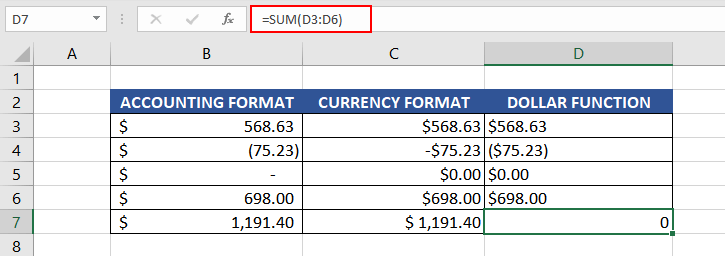
The negative values in the accounting format are displayed in parentheses like the DOLLAR function, while the currency format uses a basic format displaying the minus sign. It is also important to note that zero (0) is also displayed in different formats, as seen in row 5. The accounting format displays the value as a dash (-), and both the currency format and DOLLAR function output shows it as $0.00.

The common feature among them is that the currency symbol used with the values is dependent on the default local language settings of the computer. We can manually change the currency symbol using the Number format in Excel or directly change the windows settings.

Hopefully, the article enhanced your knowledge about the DOLLAR Function. Practice on your own and discover new applications of the function in your day-to-day life. We shall be back with more Excel tutorials to help you out.