Excel HSTACK Function – How To Use

The HSTACK function in Excel combines several arrays or cell ranges into one by stacking them horizontally. Each additional array is placed to the right of the previous array.

The HSTACK function provides us with the ability to create a consolidated dataset that meets our specific needs by selecting and combining data from multiple datasets.

Syntax

The syntax of the HSTACK function is straightforward and follows the following format.

Arguments:

The HSTACK function accepts the following arguments:

'array1' – This is the first and the only mandatory argument. It accepts the value of the first cell range or array to be horizontally combined.

'array2' – This is an optional argument that accepts the cell ranges or arrays that will be appended with array1.

All the proceeding arguments include cell ranges or arrays that will be combined.

Important Characteristics of the HSTACK Function

As the HSTACK function merges data in a column-wise fashion into longer rows. The number of rows in the resulting dataset is the maximum row count among all the input array arguments. Apart from this, some of the noteworthy characteristics of the HSTACK function are as follows.

• The number of columns in the resulting dataset is the total number of columns from each of the array
• The resulting array from the HSTACK function is completely dynamic. This means that if any data within the input array is modified, the resulting array will automatically be updated accordingly.
• If there are empty cells within the input array, the HSTACK function returns zeros instead of empty cells.
• If the value of the first argument array1 is empty, the HSTACK function returns a #VALUE! error.

Examples of HSTACK Function

The HSTACK function is an excellent tool for merging and organizing data according to our specific needs. Here we have taken diverse inputs to understand the basic work of the function in an effective manner.

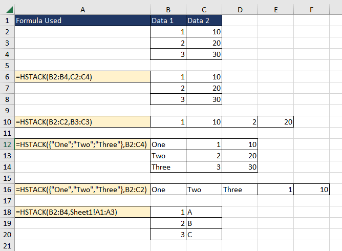
The first example is a classic representation of the HSTACK function where we are merging two ranges (columns) B2:B4 and C2:C4 horizontally. The result is data from the B2:B4 followed by all the values from C2:C4 in a single dataset.

In the second example, we are combining the data from the rows which means merging the ranges B2:C2 and B3:C3 horizontally into a single array.

The next example showcases combining a constant array containing the values "One", "Two", and "Three" (in column format) with the cell range B2:C4. The resulting dataset contains three columns, with the first column containing the values "One", "Two", and "Three" followed by the values from B2:C4.

The subsequent example displays the same functionality of combining a constant array but in row format.

The last instance displays another useful application of the HSTACK function which is combining data from different worksheets.

Now that we understand the core functionality of the HSTACK function, let's explore some additional cases for the function.

Example 1 – Simple Use of HSTACK Function

In this example, suppose you work for an electronics store that maintains three separate datasets containing information about the products, their sales, and their suppliers. Your intent is to combine the datasets to create one exhaustive database.

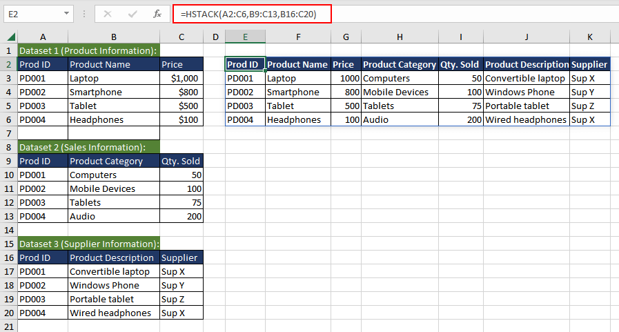
Using the HSTACK function, we would be able to combine all three datasets horizontally giving us an overview of all aspects of the product.

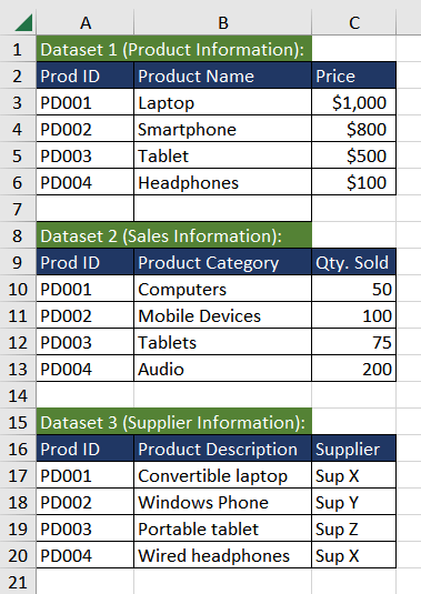
The formula used will be as follows.

The first dataset which lies in the range A2:C6 contains basic information about the product such as ID, product name, and price will be horizontally stacked with the second database which contains sales information. As the first column of the second database is a repetition, we will omit it and combine B9:C13. The third dataset also contains a duplicate column, therefore while combining, we skip it.

When working with different datasets, it is common for each dataset to have varying sizes. Now, let's explore the functionality of the HSTACK function and how it handles the combination of datasets with different sizes.

Example 2 – Combining Different Size Array with HSTACK Function

In this example, suppose we have an online website to sell shoes. We have two lists of customers, one list of customers who have purchased shoes from your website in the past month and one list of customers who have visited your website in the past month. Now, we wish to combine both lists.

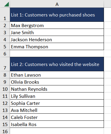
 To combine both lists horizontally, the formula used will be as follows.

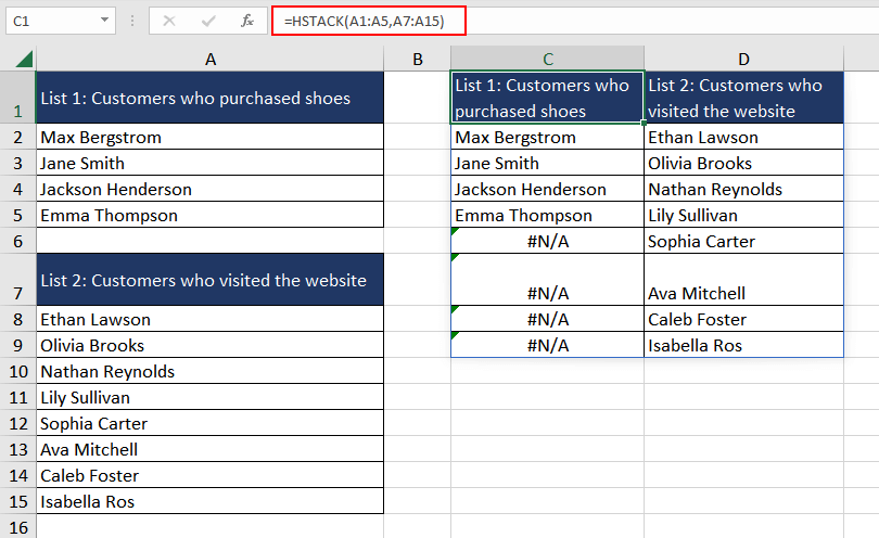
As the arrays combined are of different sizes, the HSTACK function pads the smaller array with the #N/A error to match the larger array. To remove the error, we can wrap the HSTACK function with the IFERROR function. The function used will be as follows.

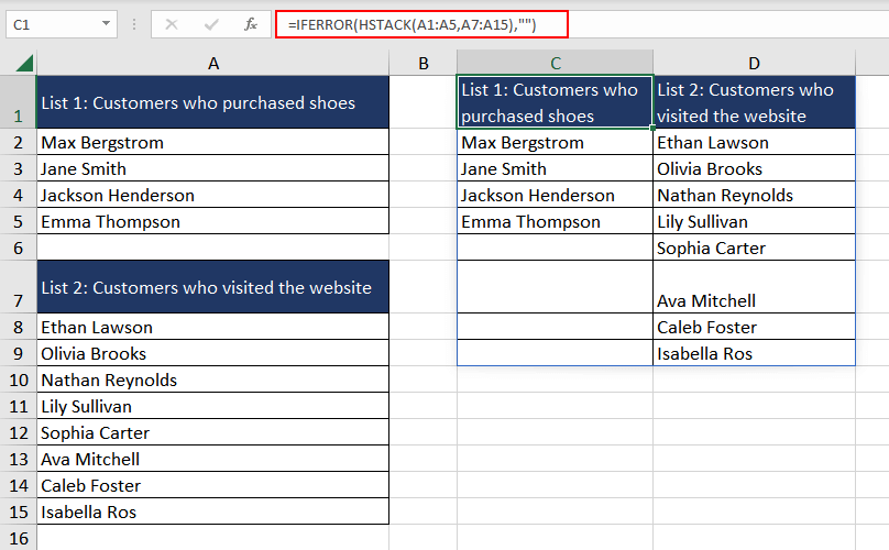
Depending on the case, you can choose to fill the empty cells with the desired data.

Example 3 – Using UNIQUE Function with HSTACK Function

In this example, we downloaded information about the FIFA World Cup history from the years 1998 to 2022 from the internet. It contains details about the winners, runners-up, third-place finishers, and host countries for each of the mentioned World Cups. As it is downloaded, it is in three separate tables.
We now wish to combine them into one to be able to use them further.

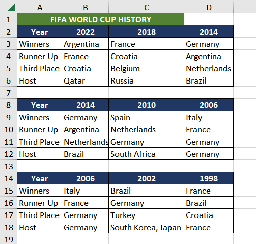
The formula used will be as follows.

Now the problem with above formula is that, some of the columns are duplicates, which is less than ideal. To resolve that, we can use the UNIQUE function to get the desired dataset. The formula used will be as follows.

By setting up the second argument of the UNIQUE function to TRUE, we are indicating it to compare the data across columns.

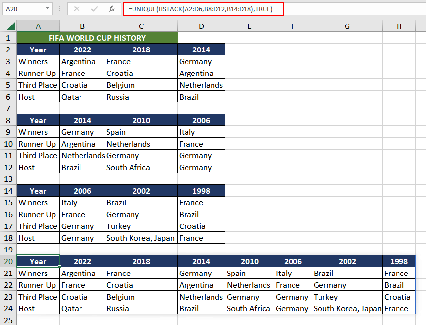
Now we have the consolidated database with no duplicates. We can go a step further and sort the data using the SORT function depending on the requirement.

HSTACK Function vs VSTACK Function

Now we know that the HSTACK function enables us to merge data horizontally, combining columns one after another. Conversely, the VSTACK function combines datasets vertically, stacking rows on top of one another.

To have a better understanding of the contrast, let's take a simple example where we have two cell ranges B1:B2 and C1:C2. The formulas used will be as follows.

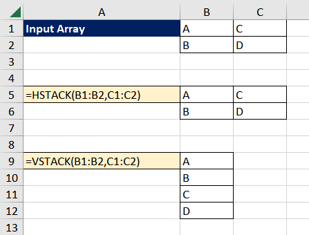
As we can see, the HSTACK function merged the data from cell ranges B1:B2 and C1:C2 horizontally while the VSTACK function combined it by stacking them on top of each other. Depending on the intended dataset, we can choose to use either one of the functions.

Practice and discover new ways to use the HSTACK function to level up your Excel skills. As you delve deeper into its applications, we will host another function to expand your Excel toolkit.