Excel HYPERLINK Function – How To Use

The HYPERLINK function in Excel allows you to create a clickable link enabling easy navigation to a specific cell, range, or Named Range within the same or a different worksheet, to a file or folder in your computer, or even directly to a web address.

The HYPERLINK function is an excellent tool to create a table of content or easy navigation when working with several worksheets or workbooks.

Syntax

The syntax of the HYPERLINK function is as follows.

Arguments:

The HYPERLINK function accepts two arguments which are as follows.

'link_location' – This is a mandatory argument that includes the target location of the hyperlink. It can be a cell reference within the same worksheet or another worksheet in the workbook. It can also be a file path or a web URL enclosed in quotation marks.

'friendly_name' – This is an optional argument that includes the display text of the hyperlink. If the value of the friendly_name is left empty, the default value is the input value of the link_location If the value of the argument is text, it must be enclosed in double quotes.

Important Characteristics of the HYPERLINK Function

Some of the notable features of the HYPERLINK function are as follows.

• To generate a hyperlink to another cell or worksheet, the value must be prefixed with the hash symbol "#".
• To select a cell containing the HYPERLINK function without following the link, you can use the arrow keys on your keyboard or right-click.

Examples of HYPERLINK Function

The HYPERLINK function proves to be highly advantageous when dealing with multiple worksheets or extensive databases.

In Excel, a convenient way to create hyperlinks is by using the keyboard shortcut Ctrl + K. Now, let's examine a few instances to gain a clearer comprehension of how it can be applied.

Example 1 – Simple Use of HYPERLINK Function

Here we have taken varied inputs for both the arguments of the HYPERLINK function to gain a better understanding.

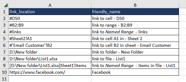
In this example, column A contains the input values for the first argument while column B includes the name that will be displayed for the hyperlink. The formula used will be as follows.

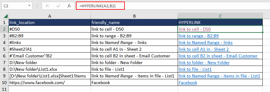
In the first case, using the HYPERLINK function we are trying to create a link that navigates the user to a specific cell within the same worksheet. It is important to use the hash symbol "#" before the cell address. Clicking on the link in cell C2, the user will be taken to cell D50 directly.

In the next example, we have created a link leading to a range. Clicking on the hyperlink in C3 will select the range B2:B9 on the sheet. This example is followed up by a hyperlink to a Named Range on the sheet. The Named Range covers cells C2 to C9.

The fourth example creates a hyperlink leading to a specific cell (A1) in another worksheet (Sheet2). This can be very useful when creating easy navigation across various worksheets like a table of content.

Next, we show you how to enter a link location of a sheet name with a space or special character. Simply enclose the sheet name in single quotation marks. E.g. the sheet name Email Customer will be added as 'Email Customer'. Then proceed with the exclamation mark and cell reference.

The following three examples demonstrate how hyperlinks can be used external to the current workbook. First is a simple folder path that you can copy and paste from your file browser (shown in row 7 of our example). To add a file name to a folder path, add a backslash and copy-paste the file name along with the file extension (e.g. xlsx, jpeg, etc.).

To further this, see row 9 where you can add the sheet and cell reference. For that, first enclose the file path in square brackets, add the sheet name ending in an exclamation mark, and then simply add the cell reference, range, or (as we have done) Named Range. The Named Range in this instance is called 'items'.

The last example is a prime example, and probably one you are most familiar with, of how to create a hyperlink to a website where the website URL is the input value of the first argument.

Notes:

For navigation within the workbook, we need to use a hashtag at the beginning of the location.

Helpfully enough, a cell, range, or even a Named Range can be selected on another sheet in the workbook and also in other workbooks (as explained above).

Now that the basic use cases of the HYPERLINK function are clear, let's explore more applications of the said function.

Example 2 – Using VLOOKUP with HYPERLINK Function

Suppose there is a job opening at the company and you are the HR. You have shortlisted a few candidates based on the preliminary requirement and now you must consolidate the list of individuals who have qualified for the next round. The dataset contains the candidates' names and the links to their LinkedIn profiles.

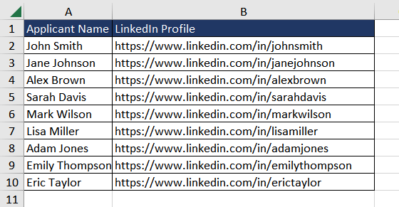
To improve the experience for the hiring manager, we can create hyperlinks that directly navigate to each employee's profile based on the name entered. We can use a combination of HYPERLINK and VLOOKUP functions where when the hiring manager enters the applicant's name, the formula creates a clickable hyperlink leading to the individual's LinkedIn profile.

Let's take cell D2 where the hiring manager can enter the candidate's name. Then, the first step is to use the VLOOKUP function for the value in D2 within the cell range $A$2:$B$10 which is the table containing applicant names and LinkedIn profile links. The formula used will be as follows.

The formula returns the corresponding value from the second column (i.e., column 2) of the range. The FALSE parameter ensures an exact match is returned.

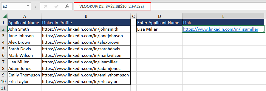
We can now use the return value of the VLOOKUP function in the HYPERLINK function where the return value is used as the first argument, whereas the second argument is the applicant's name in cell D2 which will also be the display name for the hyperlink. The formula will be as follows.

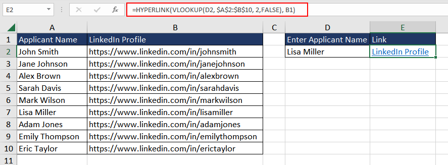
Now the hiring manager can directly navigate to the LinkedIn profiles of the required applicants.

Example 3 – Using INDEX MATCH with HYPERLINK Function

In this example, imagine you have sales data containing the performance of different products in various regions. Usually, such datasets are large, and it is difficult to find the required data. In this case, we wish to find the cell location containing the highest sales value within a specific region.

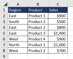
We will use the HYPERLINK function to create a clickable link leading to the cell containing the highest sales value in a particular region, let's say East. We will first use the IF and MAX function to find the highest sales value in the region "East". Then, we will use the INDEX and MATCH functions to get the cell containing the highest value. Using this data, we will create a hyperlink leading to the required data.

Let's formulate the logic in a step-by-step manner.

We will use the IF function to check if the value in column A is "East". If yes, it will return the corresponding sales value from column C. We will then wrap it with the MAX function which will return the highest sales value in the "East" region. The formula used will be as follows.

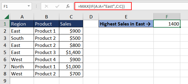
In the next step, the MATCH function looks for the highest sales value from the previous step within the sales column (column C) and returns the position of the matching cell.

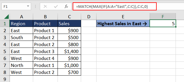
The INDEX function now takes the sales column (column C) and the row number returned by the MATCH function to retrieve the cell containing the highest sales value in the "East" region. The formula will be as follows.

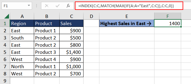
The next step is to use the CELL function to retrieve the address of the cell containing the highest sales and then concatenate it with the "#" hash symbol to create the hyperlink destination.

The final step is to wrap all the above steps in the HYPERLINK function along with the link text "Click Here for Highest Sales (East)". The updated formula will be as follows.

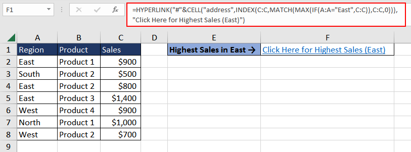
By clicking on the hyperlink in cell F1, you will be directly taken to the cell containing the highest sales value in the East region.

Example 4 – Sending Email using HYPERLINK Function

Suppose you manage a sales team and keep a record in Excel to track customer inquiries about product availability or delivery. The dataset includes customer names, email addresses, salespersons' email addresses, product names, and the status of the products. Whenever a team member receives an update, they email the customer to keep them informed.

To improve the process, the aim is to create clickable email links for each customer's email address along with the details about the product update. This will minimize the manual effort to email each customer.

We can simply use the HYPERLINK function along with the "mailto:" link. We can use other variables such as "&cc=", "&subject=" and "&body=". The formula will be as follows.

The formula creates a hyperlink to open a new email message in the default email client with the customer's email address pre-populated as the recipient and the salesperson as a cc recipient. The formula also adds the "subject" and "body" parameters to the email link.

By clicking on the email link in column F, we can quickly communicate with the respective customer and provide them with relevant product updates. The prefilled subject line, CC recipient, and email body save time and effort while enabling efficient communication and customer service.

Explore the HYPERLINK function further to enhance the usability and navigation of your Excel workbooks. Practice while we bring to you another interesting Excel function as an addition to your knowledge base.