Excel N Function – How To Use

The N function in Excel converts any input value to a number. The numeric values and errors remain unaffected, while all other data gets converted to numbers.

The N function is very useful when we strictly wish to work with numeric data and create compatibility with other spreadsheet programs.

Syntax

The syntax of the N function is as follows.

Arguments:

The N function only accepts one argument making it a mandatory input.

'value' –  This argument accepts the input data that we wish to convert into a numeric value. It can be a direct value, a cell reference, or a function that returns a value we intend to convert.

Important Characteristics of the N Function

Some of the noteworthy features of the N function are as follows.

• When the input value is boolean data, the N function converts the same into 1s and 0s.
• The N function returns the input value as it is if the data is an Excel error or a number.
• For all text data as the input value, the N function returns 0.

Examples of N Function

As the function seems to be pretty straightforward, let's explore different applications of where it can be useful with the below-mentioned examples.

Example 1 – Simple Explanation of N Function

In this example, we have taken a sample dataset as the input data for the value argument to understand how the N function behaves with different kinds of input values. The formula used is as follows.

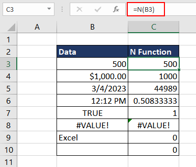
The first two examples are a classic case of the N function simply returning the number value. The N function returns the first value as it is and just removes the currency formatting from the second one, displaying the numeric value.

The next two examples are date and time as the input data for the value argument. The N function returns the numeric values of each which is the form in which Excel stores date and time.

The subsequent examples display the above-mentioned characteristics of the N function. If the value of the input data is a boolean value as is in cell B7, the return data is 1. The next example contains error data in cell B8, and as we can see in cell C8, the resulting data is without change.

The last two examples contain a text value in cell B9 and a blank cell in cell B10. For both values, the N function returns 0.

Hopefully, now you have a clear understanding of the N function and its return value for various data types.

Example 2- Identifying Text Values Using N Function

There are cases when the number values in the data are in text format due to one reason or another along with number format data. If you wish to identify the text formatted number data, the N function can be useful. For example, here in this case, we have the data containing employee names along with their salary.

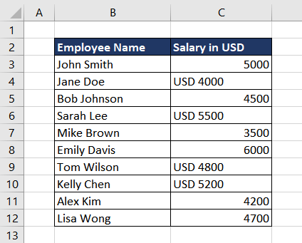
As we can see, some data in column C contains 'USD' as a prefix which makes it a text value. Now, we want to identify which values are in text format. Though it is very obvious by its left alignment, that's not an efficient way when dealing with large data.

Using the N function, we can identify the text value because when the data goes through the N function, it returns 0 for all text data. We can then add an IF function to indicate the text values.

The logic used is as follows.

IF the return value of N Function is 0, then display "Text Value", otherwise return the original value.

Let's put this in the Excel form now. The function used will be as follows.

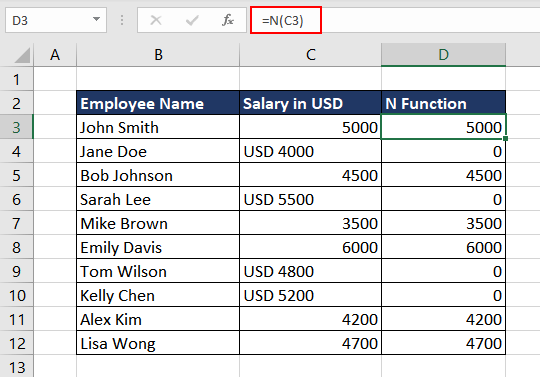
As we can see from the values in column D, the N function resulted in 0s for all the text values. Now, let's finalize the formula with the IF function, which will be as follows.

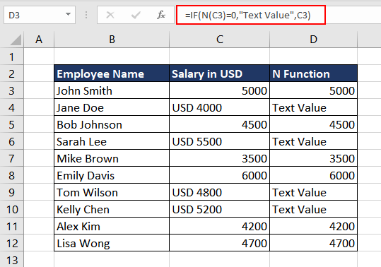
Example 3 – Counting Cells With More Than N Characters

In this scenario, we have some marketing campaign copies which must be shared online on various social media platforms. Before we forward the data, we have to ensure that the content to be published doesn't cross the maximum character limit.

We can check and count the number of cells that contain more characters than the limit using the N function combined with the SUMPRODUCT and LEN functions. Let's break down each step for better understanding.

First, we will use the LEN function to get the total character count in each cell. The formula used will be as follows.

We can also use the entire range in the LEN function, updating the formula as follows.

Let's take a cell reference where we can insert the character limit depending on the social media platform. The cell reference is F3. Now we can simply use a comparison operator to check if the return value of the LEN function is greater than F3. The formula now looks like this.

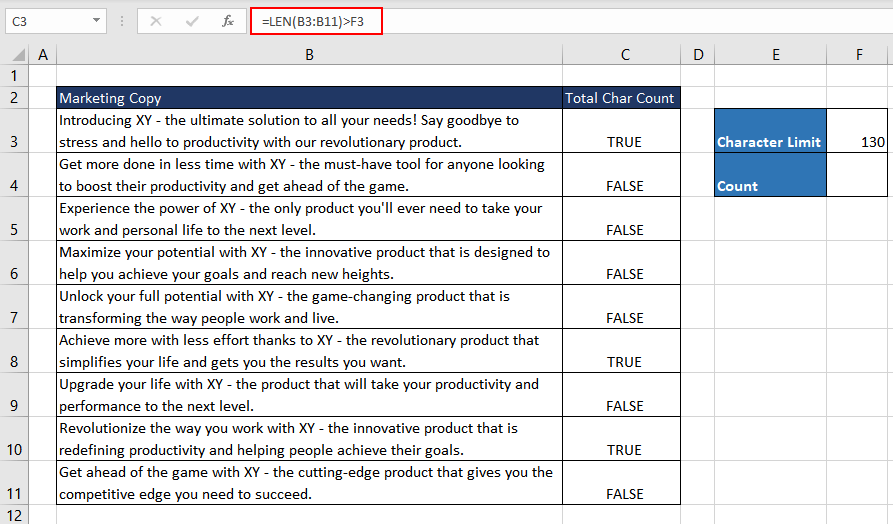
As you can see, we now have TRUE and FALSE in column C indicating which cells contain more characters than the limit. We can now wrap the above function in the N function, giving us 1s and 0s.

Finally, we can use the SUMPRODUCT function to give us the total number of cells or marketing copies in this case that contain more characters than needed. The final formula will be as follows.

Using the same logic, we can also count the number of times a month is repeated in a range of dates. Let's understand it better with an example.

Example 4 – Count Occurrences of Months in Range of Dates

In this example, we have the dates on which one of the employees is taking leaves. For better resource planning, we want to check how many days fall in the same month.

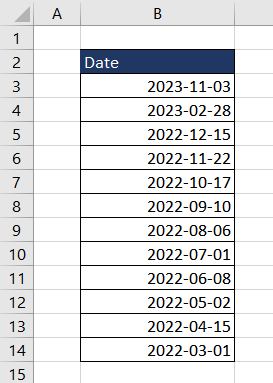
Using the MONTH function, we can extract the month from the dates in column B. We can then compare the extracted months with the month we wish to check and then calculate the sum of all TRUE values.

To compare the months from column B with the month we wish to compare with, which is in cell E3, the formula used will be as follows.

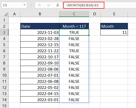
So, here we are checking what's the occurrence of month 11 in the range of dates. Now that we have the TRUE and FALSE values, we can use the N function to convert the boolean values into 1s and 0s.

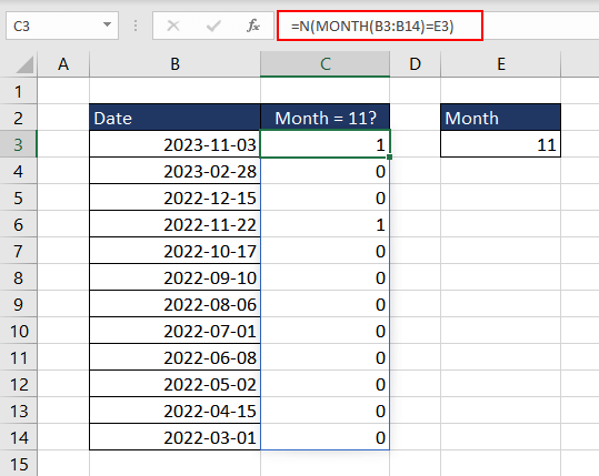
Now, we can wrap the function in the SUMPRODUCT function to get the total count. The final formula is as follows.

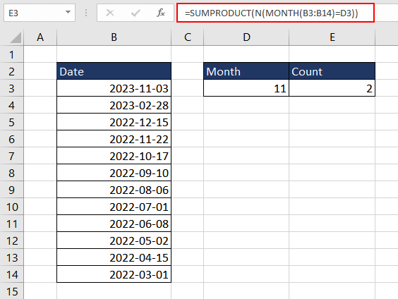
Example 5 – Leaving Comment in Formula

Another application of the N function is to leave a comment in a cell that returns a numeric value. Let's see how to do that using an example. Here, we are simply calculating the average of values in column B. So the formula used will be as follows.

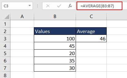
Now, if we wish to leave a comment here for better understanding, we can add the N function along with the above-mentioned AVERAGE function. For that, we will use the comment as the input value for the N function. The formula used will be as follows.

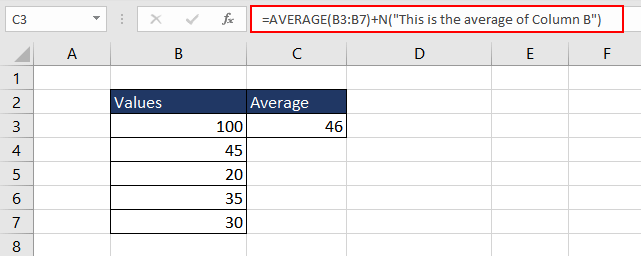
Whenever the user clicks on cell C3, they can see the comment. And we could accomplish it without altering the numeric value in the cell. The reason is that the N function returns 0 for all the text values and the resulting numeric value from the first function simply adds 0, therefore no alteration in the final result.

N Function vs T Function

As we have already established, the N function is a numeric identifier and is used to convert any value to numeric data. The T function on the contrary is a text identifier. The T function only returns the input value if it's text data, else it returns an empty string.

The N function either returns the numeric value of the input data or returns 0. These are the only two functions in Excel whose names contain one character only and are very useful for dealing with big datasets.

We hope this Excel function helps you enhance your efficiency when working with large amounts of data. As you continue to work with Excel, remember to incorporate this function into your workflow while we work on more tutorials and tips to help you master Excel.