Excel DAYS Function – How To Use

The DAYS function, categorized as a Date/Time function, is a worksheet (WS) function that allows us to compute the number of days between any two given dates. The DAYS function saw the light of day with MS Excel 2013, so if you are on an older version, you will need to rely on the DATEDIF function instead.

Syntax

The syntax of the DAYS function is as follows:

Arguments:

end_date – This is a required argument where you may supply either a serial number of date or refer a cell containing a date. Note that the date must fall after the date entered in the start_date argument; otherwise, your return will be negative.
start_date – This is a required argument where you may supply either a serial number of a date or reference a cell containing a date. Intuitively enough, the date in this argument must fall before the date entered in the end_date argument; otherwise, your return will be negative.

Important Characteristics of the DAYS function

• The DAYS function will subtract the second argument from the first argument, so you will want to enter serial numbers or cell references bearing this in mind.
• If you wish to supply dates as a text string in the DAYS function’s arguments, be sure to include double quotes (""). Excel will interpret these strings as DATEVALUE("date_text") and then compute the output for the DAYS function.
• The DAYS function will return a #NUM! error if the arguments are supplied as serial numbers, and the serial numbers are not within the range of valid dates.
• The DAYS function will return a #VALUE! error if dates supplied as text strings in either or both arguments cannot be parsed as valid dates.

Examples of the DAYS function

Now let's have a look at some of the examples of the DAY function in Excel.

Example 1 – Plain-vanilla DAYS function

Let’s start with the simplest form of DAYS function. We will use all three methods of supplying arguments to the DAYS function. However, the formula’s structure will remain unchanged:

In the above example, the first formula uses cell references A2 and B2 as the arguments to the DAYS function. The cells A2 and B2 contain dates and the resultant is the difference between the given dates in days.

The second formula uses cell references A3 and B3 as the arguments to the DAYS function. The cells A3 and B3 contain serial numbers and we know that Excel internally treats dates and serial numbers so the DAYS function accepts them, and the resultant is the difference between the two numbers.

Additionally, the DAYS function can also accept dates as text values, as shown below:

Naturally, the simplest way to do this is either referencing the cells or entering text strings, but serial numbers are included just for clarity.

Example 2 – Tackling Negative Values

Let’s address the elephant in the room. What if you have a list of dates in two columns such that some rows have the start date in column 1, while other rows have the start date in column 2, and you want the number of days between those two dates?

Enter the ABS function.

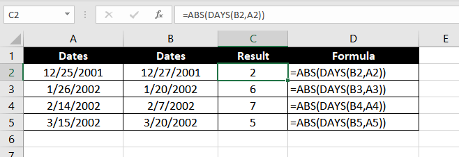
The ABS function returns the absolute value of any number in a given cell. To apply the ABS function, we will use the following formula:

Since the DAYS function returns a negative value when the end date falls before the start date, the ABS function removes the negative sign and gives us the absolute value. This is the same output you would receive if you interchanged the position of start date and end date manually. Therefore, this formula saves you a ton of labor.

Example 3 – Calculate the Number of Days Daily

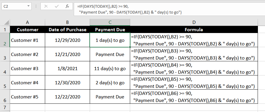
Let’s say you are a B2B organization that sells goods on credit. In the example, we have a list of dates on which we made a credit sale to our customers. We have a 90-day credit policy, which means we must contact buyers who have not paid their invoices once 90 days elapse from the date of sale.

In this case, we want to find out the number of days since the customer has made a purchase. To do this, we can use the following formula:

The formula that we have used sets the end_date argument to today’s date using the TODAY function. The start_date date argument is set to the date of the last sale, and thus DAYS function calculates the number of days since the last sale was made.

Let's take this formula to the next level, and instead of calculating the number of days, let's try to mark all the customers for which the payment is due with a text that says "Payment Due" and for all other customers, we will set a text that says how many days are remaining for the payment due date.

We can do this using the IF Function, and the formula will be:

This formula uses the DAYS function along with the IF function to display a result based on the return from the DAYS function. If the return from the DAYS function is greater than or equal to 90, then it shows a message saying "Payment Due" otherwise, it calculates the difference between 90 and the result of days function and shows a message "XX day(s) to go".

Example 4 – Building Logic to Find Out a Leap Year with DAYS function

Now let's try to solve a practical problem with the DAYS function in excel and try to build a formula that determines if the given year is a leap year or not.

We know that a leap year has 366 days, and we can make use of the DAYS function to count the number of days in the specified year. With an IF function, we can check – If the resulting number is equal to 366 or not. If the number is equal to 366, we can mark the year with the text "Leap Year"; otherwise, another text, "Not a Leap Year" can be displayed.

So the formula would be:

In the above formula, we are using three functions – DATE, DAYS, and IF function.

The job of the DATE function is quite simple. It helps in generating the arguments for the DAYS function. For example – if the given year is 2010, the DATE function would generate the end_date as 12/31/2010 and start_date as 12/31/2009.

Next, the DAYS function comes into the picture. It will calculate the difference between the dates generated above.

Finally, with the help of an IF function, we are checking the result of the DAYS function. If it is equal to 366, then we mark the year with the text "Leap Year"; otherwise, another text, "Not a Leap Year" is displayed.

That sums up the DAYS function. A simple, powerful function that helps us play around with dates on our worksheet. Take a few stabs at the DAYS function, and revisit the tutorial if you need it. When you are done, we will have some more intriguing formulas and another handy function for you to excel in.