Excel INDEX Function – How To Use

The INDEX function enables us to retrieve specific data from a range of cells or arrays based on the row or column position. In this data-intensive world, the INDEX function is one of the most talked about functions in Excel.

It is mostly used when navigating through large datasets and setting up dynamic extractions or ranges. If you know the location of the required data within the dataset, the INDEX function can easily retrieve the value for you.

Syntax

The INDEX function in Excel has two distinct syntaxes, with the second syntax incorporating an additional argument. Depending on the need of data retrieval, users can choose the input values accordingly.

For the array form of the INDEX function, the syntax is as follows:

The second one is known as the reference form as it allows the user to choose which cell reference to extract data from:

Arguments:

'array – This is a mandatory argument that includes the cell range or array from which we intend to extract data. The value of the array argument can also be an array constant.

'reference' – This mandatory argument is used when we have more than one cell range. It includes the value of cell references to ranges from which we wish to extract the data. If the cell ranges are non-adjacent, the values must be enclosed in parentheses.

If the input value of the array or reference argument contains only one row or column, the subsequent row_num or column_num arguments are optional.

'row_num' – This argument indicates the row number from which we wish to extract the date from. The input value of the row_num must be a positive integer. If the column_num argument is skipped, this becomes a mandatory argument.

'column_num' – This argument holds the value of the column number which contains the data we wish to retrieve. If row_num is omitted, column_num is a required argument.

When the values of both row_num and column_num arguments are mentioned, the INDEX function will return the value at the intersection of the specified row and column.

'area_num' – This is the last argument of the reference form of the INDEX function. This argument indicates which cell ranges to extract the data from when there are multiple cell ranges. The default value of the area_num argument is 1.

Important Characteristics of the INDEX Function

Some of the noteworthy features of the INDEX function are as follows.

• When the value of both the arguments row_num and column_num are set to 0, the INDEX function simply returns the input array or cell range.
• If the value of row_num or column_num is a negative number, the INDEX function returns a #VALUE! error.
• The INDEX function returns a #REF! error when the value of row_num, column_num, or area_num arguments does not point to any cell within the input array or reference.
• When using the reference form of the INDEX function, all input cell ranges must be in the same sheet, else the INDEX function throws a #VALUE! error.

Examples of INDEX Function

Let's begin by understanding the core functionality of the INDEX function. Here we have taken a basic dataset and will use varying input values for all the arguments to gain a better understanding.

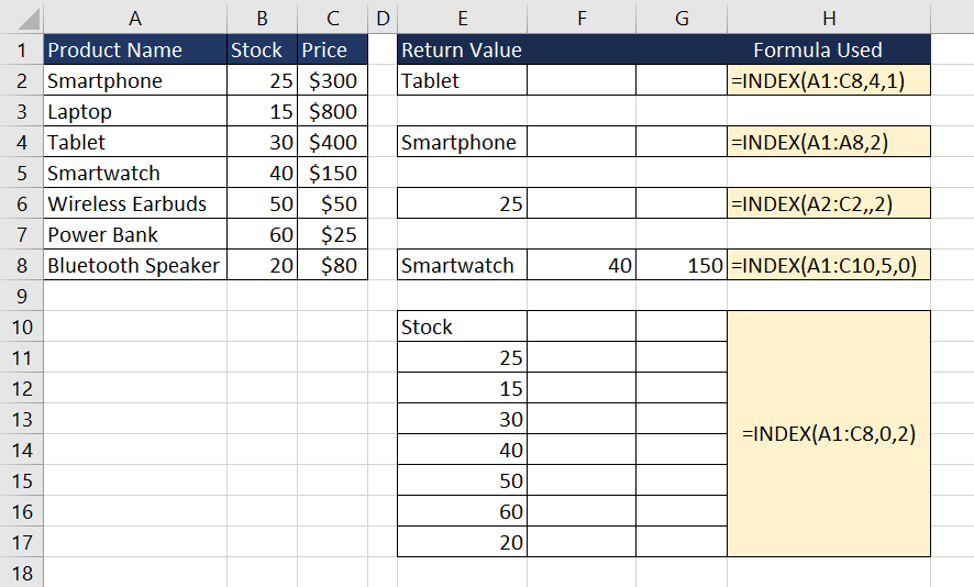
The first example is a classic case of the INDEX function where we have a two-dimensional array or cell range (A1:C8) and the intention is to retrieve the value at the intersection of the 4th row and 1st column. The return value is "Tablet", as intended.

The next two examples show the case when the input cell range or array is one-dimensional. In such cases, we can use one of the arguments. In the second example, we are extracting data from the second row of the cell range A1:A8, while in the third we want the data that is in the second column of the cell range A2:C2.

The last two examples explore how the INDEX function works when the value of either row_num or column_num is set to 0. In these cases, the entire row or column is returned.

These examples showcase the flexibility and power of the INDEX function when dealing with data retrieval tasks. Let's explore more examples to gain a deeper understanding of the INDEX function's capabilities.

Example 1 – Simple Use of INDEX Function

Suppose you are planning an outing to the beach and wish to decide which day is the most appropriate depending on the weather. You downloaded the weather report for the next month starting from day 1. The data contains different weather-related details for each day. Now, you wish to retrieve the weather-related information for a specific day by specifying the day number.

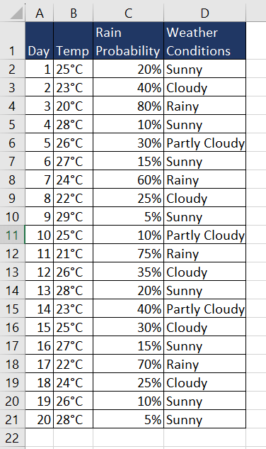
This example showcases an elementary application of the INDEX function, allowing us to fetch a specific value from an array based on a particular position.

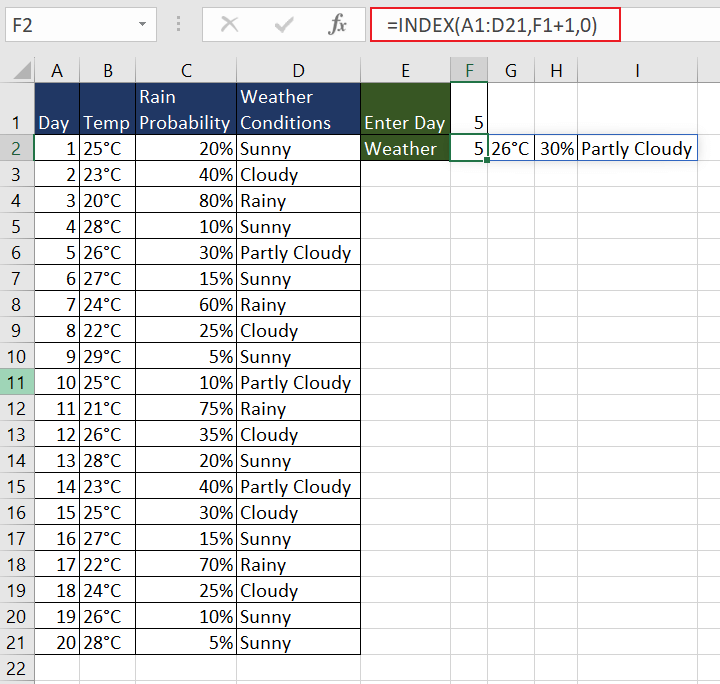
For instance, by utilizing cell F1 as a reference for the day number input, we can dynamically fetch the corresponding weather information using the INDEX function. The formula used will be as follows.

This function retrieves the value in row number F1+1 from the array A1:D21. We are adding 1 to accommodate the first row which is used as header. As the column_num is set to 0, it will return the entire row giving us all the weather information for the given day.

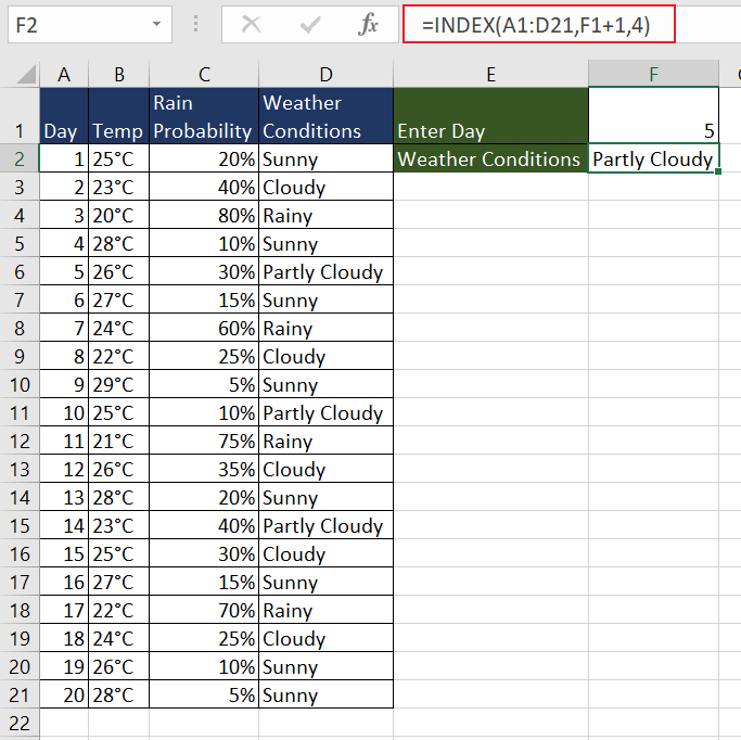
Now, what if we just want the weather conditions for a particular date? The formula used will be as follows.

Instead of 0, we have entered the argument for the column number as 4 since the column for weather conditions is the 4th column in the array.

Example 2 – Using Reference Form of INDEX Function

In this scenario, we have the sales data of a company for three consecutive weeks in separate datasets. The goal is to efficiently extract the sales data for specific dates from a chosen dataset.

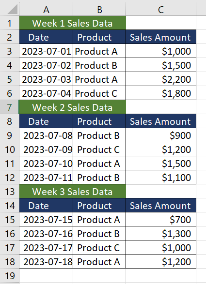
One way is to use the INDEX function separately for three datasets. A more efficient way is to use the reference form of the INDEX function. When using multiple cell ranges, we can enclose them in parentheses separated by commas such as (A3:C6,A9:C12,A15:C18) for all three weeks.

Let's say we wish to retrieve 2nd day's data from week 2. The formula used will be as follows.

As we want to extract the entire row, we will leave the column_num argument empty. To ensure that the data is extracted from the second dataset, we will assign the value of area_num to 2.

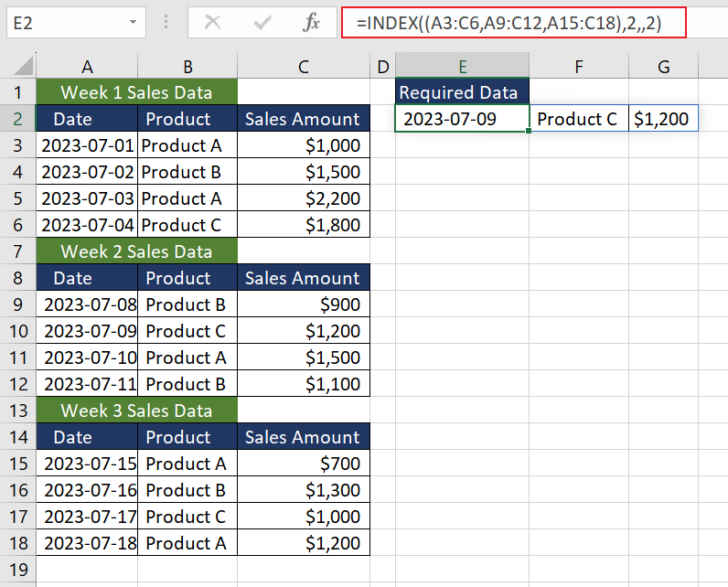
There is no need to join separate datasets before retrieving the desired data.

Example 3 – Creating Dynamic Ranges with INDEX Function

As the electricity prices have gone up, we wish to analyze the average consumption among other things to find sustainable ways to optimize consumption and cost. We have the data for monthly electricity consumption where each row contains different months' data, while the columns include data such as electricity consumption, cost per kWh, and total cost.

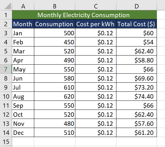
One way to calculate the average consumption is to use the AVERAGE function and manually add the cell ranges. A more efficient way is to use the INDEX function to create a dynamic range based on the user's input.

The idea is to calculate the average of a range of values in column B, starting from cell B3 where the ending point of the range will be determined dynamically using the INDEX function.

We will take cell G1 where the number of months for the average calculation is entered. This value in G1 will also indicate the row number parameter for the INDEX function, allowing for a dynamic range selection. The formula used will be as follows.

We are adding 2 to include additional rows in the range which are headers in the dataset. Now, adding the AVERAGE function, the formula will be as follows.

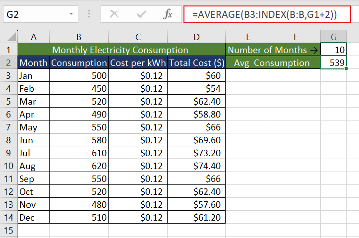
When dealing with larger datasets, it is smart to create a dynamic range to be able to retrieve data faster.

INDEX and MATCH Functions

When looking for data within a dataset, the most commonly referred function is VLOOKUP. However, the VLOOKUP function has a few limitations such as the lookup column must be on the left side of the return column. To overcome that limitation, use the XLOOKUP function (available to MS 365 and Excel 2021 users). Otherwise, a combination of INDEX and MATCH functions is recommended.

The INDEX function allows us to extract specific data from a dataset when we know the exact location. To complement its capabilities, we have the MATCH function, which helps us find the precise location of data within the dataset. By using a combination of INDEX and MATCH functions, we will be able to perform dynamic lookups. Let's understand it with an example.

In this case, we have a dataset that contains employee IDs, updated salary details, and additional employee information. Now, the user wishes to extract all employee information based on their Employee ID.

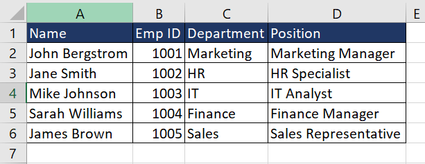
The MATCH function finds the position of the required data in the table and then the INDEX function returns the value from that position. Let's take cell G1 where the user can enter the Employee ID.

The MATCH function will look for an exact match of value in G1 in column B. The formula used will be as follows.

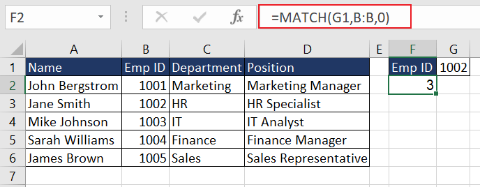
Now the INDEX function can retrieve the corresponding Name, Department, and Position from columns A, C, and D, respectively, based on the row number found by the MATCH function. We will use the return value of the MATCH function as an input value for row_num in the INDEX function.

Also, because we wish to extract all employee information, we will leave the column_num argument empty. The formula used will be as follows.

That's all from us on the bright qualities of the INDEX function and its ability to retrieve target information from throngs of data. Next time you're faced with data lookup tasks, do recall the INDEX function. Meanwhile, we're buffing up another function gem to bring its shiny facets to you. Trick on, folks!