Excel TEXTBEFORE Function – How To Use

The TEXTBEFORE function returns the text that occurs before the given character or string. That character or string is known as a delimiter. We can also decide to extract the content before a specific delimiter occurrence if the delimiter is used more than once.

The TEXTBEFORE function is a new addition to the Excel family and is only available for Microsoft 365 users.

Syntax

The syntax of the TEXTBEFORE function contains six arguments and is as follows:

Arguments:

Out of the six arguments, only two are mandatory. Details and functions of each argument are given below.

'text' – This is the first mandatory argument. The input value of the text is the original string or text from which we wish to extract. It can be a direct value in double quotes or a cell reference containing the text.

'delimiter' – This is the second mandatory argument that accepts the value of a character or string before which we intend to extract the text. The value of the delimiter can be a direct value enclosed in double quotes or a cell reference.

'instance_num' – This is an optional argument with a default value of 1. The instance_num argument refers to the nth occurrence of the delimiter before which we wish to extract the text. If the value of the instance_num argument is negative, the TEXTBEFORE function looks for the delimiter from right to left.

'match_mode' – This is an optional argument that only accepts a boolean input value of 1 or 0. The default value of match_mode is 0, which makes the function case-sensitive. If the value of match_mode is set to 1, the function performs a case-insensitive search for the delimiter.

'match_end'  – This is also a non-mandatory argument and accepts boolean input of 1 or 0. The default value is set to 0. When the value of match_end is set to 1, the function assumes the end of the text as a delimiter.

'if_not_found' – This last argument is useful when the given delimiter is not found in the text. The default value is set to #N/A. The if_not_found argument accepts the value we wish to return when the delimiter is not found. It can be a direct value in double quotes or a cell reference.

Important Characteristics of the TEXTBEFORE Function

One of the elementary features of the TEXTBEFORE func

tion is that it is a text function; therefore, the return value is always in text format. Other noteworthy characteristics of the function are as follows:

• If the text argument is left empty, the function results in a #N/A error.
• The instance_num argument accepts an integer value. If the input value of the argument is decimal, only the integer part of the value is considered.
• When the instance_num argument is set to 0 or is more than the length of the input text, the TEXTAFTER function returns a #VALUE! error.
• The function results in the #N/A error when the instance_num value exceeds the number of delimiter occurrences.

Examples of TEXTBEFORE Function

As the TEXTBEFORE function accepts several arguments, understand the usage of each with the help of the examples given below.

Example 1 – Simple Use of TEXTBEFORE Function

In this example, we have taken some sample data in text and numeric format to understand the basic functionality of the TEXTBEFORE function.

The first example is a basic email ID as the input value of text where we wish to extract the username which appears before the at the rate sign (@). We will use the @ sign as the input value of the delimiter. The return value in cell C3 is "mark", as expected.

The next example is a numeric value in cell B4. Here, we are trying to extract the values before the number 5. So, the delimiter used will be "5". The return value is '1234', appearing before 5 in the original text. It is crucial to note that the return value in cell C4 is left-aligned and is, therefore, in text format.

In the last instance, you will notice an additional argument in the formula, as seen in cell D5. Here, we wish to extract text that appears before the last dot. As there is more than one dot, we can use the third argument, instance_num. When we assign the value as 3, the function returns the text that occurs before the 3rd occurrence of the dot, which is also the last in this case.

Now that the basic usage of the TEXTBEFORE function is clear let's explore additional applications using the examples below.

Example 2 – Extracting Names using TEXTBEFORE Function

In this example, we have received the list of corporate awards presented last year from the HR team. But the information is not in the form of a list. To forward the list of awardees for certification, we have to segregate the names from the string.

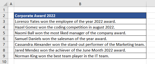
As observed, every name is followed by the word 'won'; therefore, it can be used as a delimiter, and we can simply extract the words before the word 'won'. The formula used will be as follows:

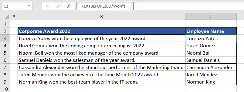
In this case, the word 'won' was common across the data. However, there is another way to achieve the same result. We can use space as the delimiter, but as there are multiple spaces in the input text, we will make use of the instance_num argument. We intend to extract the words before the 2nd space, so the formula will be as follows:

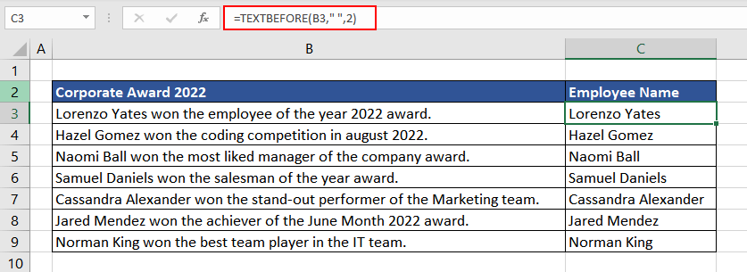
Now, using either way, we can forward the list of employees as needed.

Example 3 – Extracting Movie Names using TEXTBEFORE Function

After the Golden Globe Awards, we downloaded the list of winning movies to watch over the weekend. Upon downloading, we realized that we wish to segregate the movie names in a separate column to share them further.

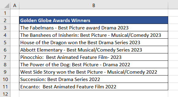
We can easily do so using the TEXTBEFORE function but the character or string separating the movie name in each case is different. In such scenarios, we can use multiple delimiters, which in this case would be a dash (-), colon (:), and the word "won".

Multiple delimiters must be each enclosed in double quotes, separated by a comma, and used as array constants in curly brackets. The formula used will be as follows:

Using this formula with multiple delimiters, we have been able to separate the movie names effectively:

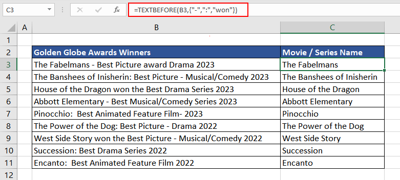
Now we have a list of movie names that we can share.

Example 3.1 – Understanding match_mode in TEXTBEFORE Function

Now, imagine if the same movie data had an inconsistent case type. Will the same formula give us the required result? Let's find out.

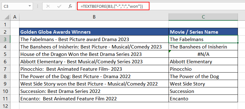
As observed in cell C5, the function returned #N/A, which is the default value when the delimiter is not found. As the TEXTBEFORE function conducts a case-sensitive comparison when looking for the delimiter, it ignores the delimiter in cell B5 as the case type is different; the delimiter in the input is "Won" instead of "won". We will assign the value 1 to the match_mode argument to make the function case-insensitive. The updated formula is as follows:

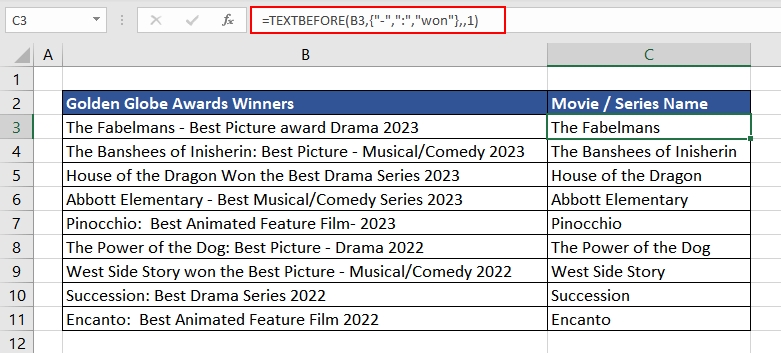
Example 4 – Negative instance_num Argument in TEXTBEFORE Function

In this case, we downloaded some simple maths questions with answers so that students could practice for the upcoming test. For better preparation, we intend to remove the answers and just extract the questions in a separate column.

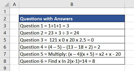
As we can see that each question is followed by an equal sign (=) and then the answer. We can simply use the equal to sign as the delimiter to extract the text before it. The formula used will be as follows:

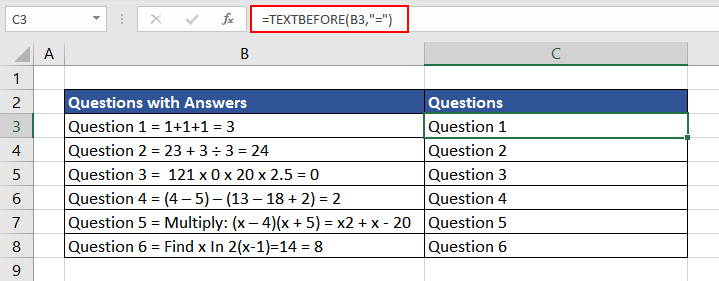
Now, the problem is by default, the TEXTBEFORE function extracts everything before the first occurrence of the delimiter. In this case, there is more than one equals sign in each question, and the last equals sign separates the answers from the questions. So, using the negative value of the instance_num argument, the formula will be as follows:

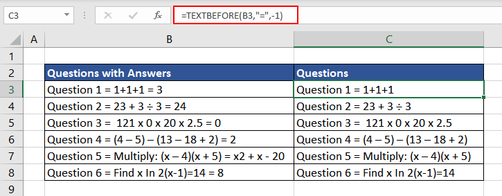
When the value of the instance_num argument is negative, the TEXTBEFORE function looks for the delimiter from right to left giving us the required data.

Example 5 – Calculating Sum using TEXTBEFORE Function

In this scenario, a courier company is delivering some goods and has sent us the details of the same. To ensure that we receive everything, we wish to count the total units we will receive.

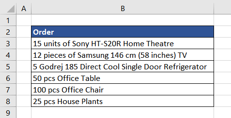
Looking at the details received, we can easily extract the text before the first space, which is the number of pieces, and then calculate the sum. The formula used will be as follows:

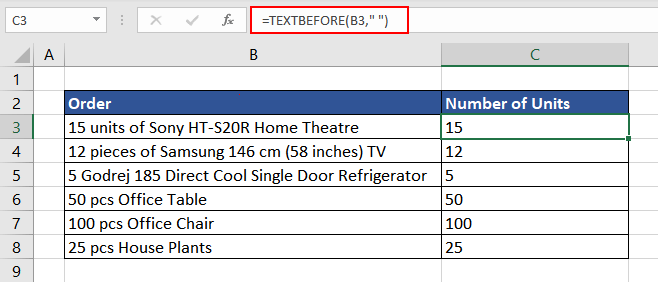
Now that we have the number of units separated in a column, we can calculate the total. But the problem is, as the TEXTBEFORE function is a text function, all the return values in column C are text values which is evident due to its left alignment.

We can use the VALUE function to convert the numbers resulting from the TEXTBEFORE function from text to number format and then calculate the total. The formula used will be as follows:

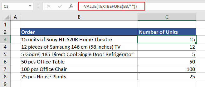
Now we can calculate the sum of cells C3 to C8. Combining all three steps and calculating the total units in one step, the updated formula looks like this.

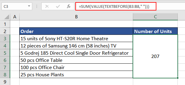
Now, you also know how to use the TEXTBEFORE function and perform mathematical calculations with the data extracted.

You now understand how to use the text, delimiter, instance_num, and match_mode arguments. The following example is designed to help you comprehend the final two arguments, which are match_end and if_not_found.

Example 6 – Missing Delimiters in TEXTBEFORE Function

In this example, we downloaded the list of the world's most powerful people as per Forbes. The list contains people's names along with their countries. We wish to segregate the names into one column.

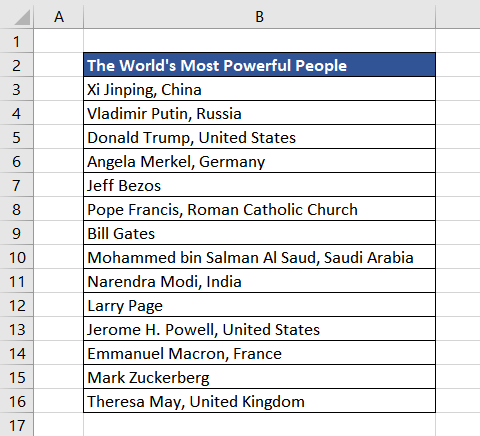
Using the TEXTBEFORE function, we can simply extract the text before the comma in each case. The formula used will be as follows:

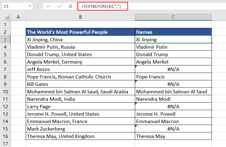
As we can see, there are a few entries where the delimiter is missing. In such cases, the function returned #N/A, which is the default value of the if_not_found argument. Instead, we can update the formula to return the original text value where the delimiter is missing. The formula will be as follows:

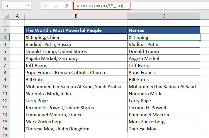
Now we have all the names in a separate column C. However, we can also achieve the same result using the match_end argument.

When we set the value of the match_end argument to 1, the function considers the end of the text as a delimiter when the given delimiter is not found. So for instances where the comma is not found, the TEXTBEFORE function will assume that there is a comma at the end of the string and return the complete text before that, which is the original value of the text. The formula used will be as follows:

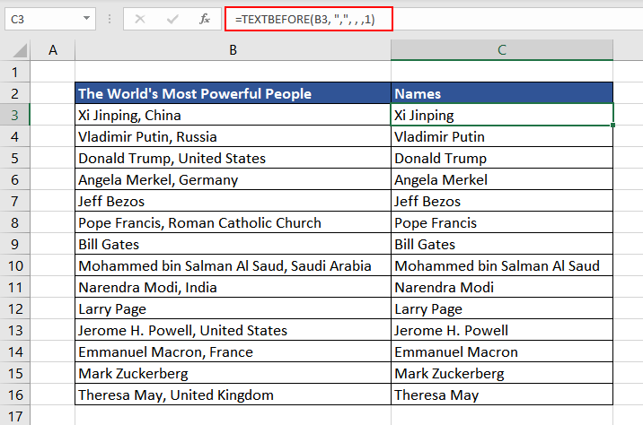
So, you can use either of the ways to get the desired result.

TEXTBEFORE Function vs TEXTAFTER Function

Like the TEXTBEFORE function extracts a part of the text which occurs before the mentioned character or string, similarly, the TEXTAFTER function pulls out the text that appears after the given delimiter, which can be any character or string. Let's use both functions in an example for a better understanding.

In this example, we have a list of full names, where we wish to extract the first and second names in separate columns.

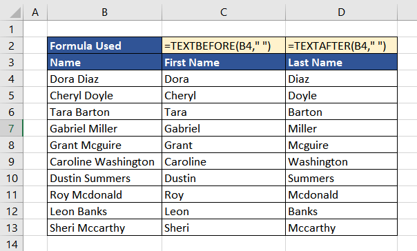
We can use the TEXTBEFORE function to extract the first name, which appears before the space, while we can utilize the TEXTAFTER function to segregate the last name as it appears after the space. The formulas used will be as follows:

Both TEXTBEFORE and TEXTAFTER functions have simplified the process of text manipulation in Excel. If you are using any other version of Excel besides Microsoft 365, then you can use the combination of the RIGHT function and LEFT function combined with the SEARCH and LEN functions to achieve similar results.

Practice the TEXTBEFORE function to discover new applications and fun ways to use it. While you do that, we will bring you another Excel function to add to your bag of tricks.