Excel VSTACK Function – How To Use

VSTACK function in Excel is used to combine multiple cell ranges or arrays in a row-wise manner. All the input cell ranges or arrays are vertically appended one after the other, resulting in a single array.

The VSTACK function is particularly useful when dealing with large data which needs to be selectively combined into one consolidated dataset.

Syntax

The syntax of the VSTACK function is as follows.

Arguments:

The VSTACK function accepts the following arguments.

'array1' – This is the first and the only mandatory argument that accepts the first array or cell range to be combined.

'array2' – This is an optional argument that accepts the cell ranges or arrays that will be vertically merged after array1.

All the subsequent arguments are optional and accept additional arrays or cell ranges to be combined.

Important Characteristics of the VSTACK Function

A standout feature of the VSTACK function is its ability to generate a dynamic array. If any modification is made to the input array arguments, it is automatically reflected in the resulting array. Other noteworthy characteristics of the VSTACK function are as follows.

• The total number of rows in the resulting array will be the combined number of rows from the input array or cell range.
• Total number of columns in the output array will be the maximum number of columns in the specified arrays.
• If the input array contains empty cells, the VSTACK function returns zeros instead of empty cells.
• If the first argument array1 is empty, the VSTACK function throws a #VALUE! error.

Examples of VSTACK Function

Here we have taken different input values for the VSTACK function to get a foundational understanding of how it operates.

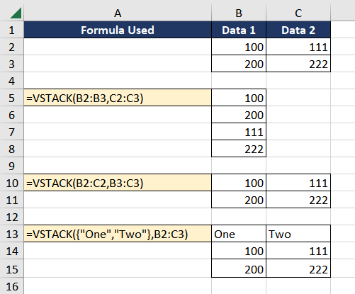
The first example is a classic example where we intend to stack two cell ranges B2:B3 and C2:C3 vertically on top of each other. As we can see, the second cell range is followed by the first as intended.

In the second example, we are merging data from two rows and wish to stack them one on another. The last example is to showcase the use of the VSTACK function to merge static arrays with cell ranges. As the static array is the input for the first argument, it goes on top of the new array, and the cell range is appended below that.

As now we know how to use the VSTACK function to combine data from different sources into a single array, let's explore different use cases to further understand the function.

Example 1 – Simple Use of VSTACK Function

Suppose you work for a company that sells products of various categories such as electronics, apparel, and home goods. Each category maintains its respective sales records; however, you wish to combine all the sales data for comprehensive analysis and reporting.

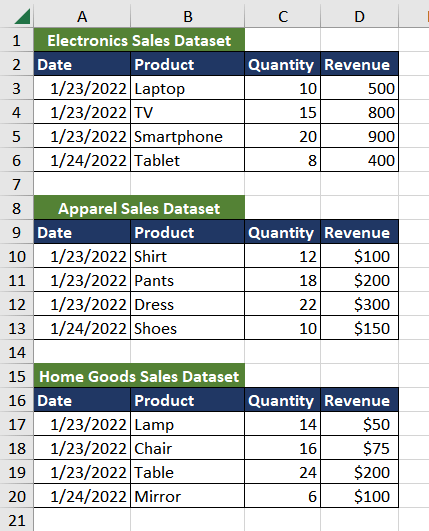
Using the VSTACK function in Excel, we can vertically merge the datasets into one. The formula used will be as follows.

We are taking the cell range A2:D6 from the first dataset. However, in the next two datasets (A10:D13 and A17:D20), we skip the first row because the heading is common across the datasets, and we want to avoid repeating it in the combined result.

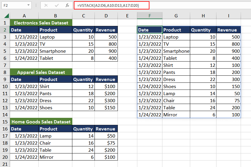
This is a classic use case of the VSTACK function where we now have the required data in a consolidated form to be used further for analysis. There can also be cases when the datasets that need to be combined vary in size.

Let's see how the VSTACK function merges datasets of different sizes.

Example 2 – Merging Different-Sized Arrays Using VSTACK Function

In this case, the company that you work for collects customer information through multiple sources such as online forms, email marketing, and social media. To be able to filter out the data and use it in a productive manner, it is important to consolidate it.

Using the VSTACK function, we can easily merge the datasets vertically.

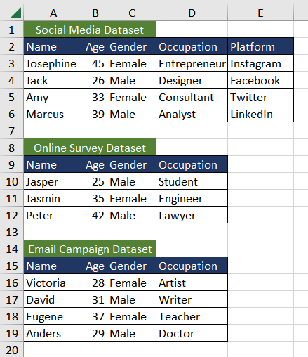
The formula used will be as follows.

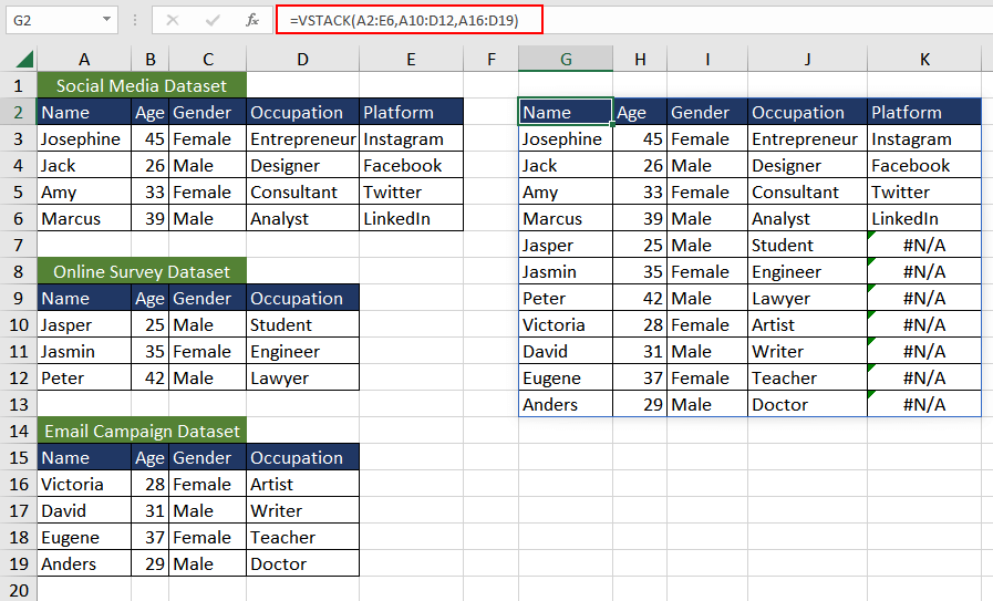
As the size of the datasets to be combined varies, the smaller array pads the empty cells with the #N/A error value. To remove this, we can use the IFERROR function to replace the error value with something relevant. In this case, we can replace it with an empty string. The formula used will be as follows.

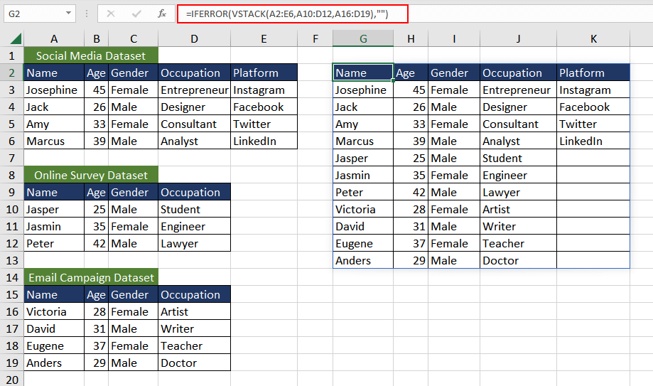
Example 3 – Combining Unique Array Using VSTACK Function

Suppose you are the sales analyst at the company and have received the sales data from both the company's website and the physical shop. You need to consolidate the data and clean it up for analysis.

Usually, such data is large and may contain duplicates, so a combination of the VSTACK function and the UNIQUE function will be useful to merge the data.

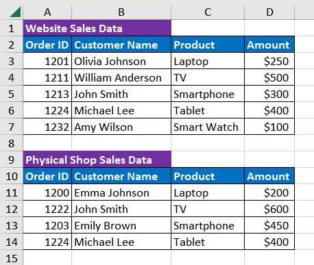
The formula to combine the sales data will be as follows.

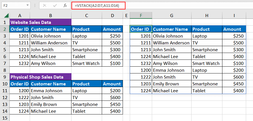
To remove the duplicates, we will use the UNIQUE function. The formula will be as follows.

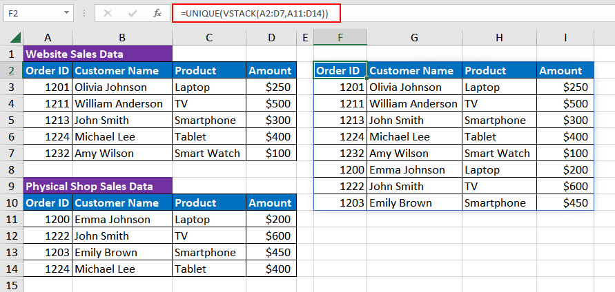
Now the data is clean. To take it a step further and arrange the data from highest sales to lowest, we can utilize the SORT function. The formula will be as follows.

The arguments added for the SORT function are 4 and -1. 4 is the column in the array that the data is to be sorted by. -1 will sort the data in descending order. Here is the data stacked, unique, and sorted:

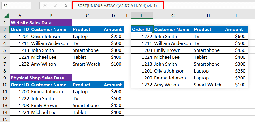
We now have the required data in place.

Example 4 – Merging Data Across Worksheets Using VSTACK Function

In this example, we have separate Excel sheets containing employee information from different departments such as employee ID, name, age, job title, salary, and performance evaluation. We now need to bring together all the data in one sheet for annual performance analysis.

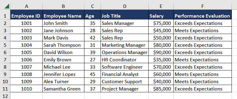
The data in all the sheets is in the same format and there are three sheets named 'Dept 1 – Sales',' Dept 2- Marketing', and 'Dept 3 – Finance'.

As the top row (column headers) is the same in all the sheets, one way is to manually copy and paste it into a new sheet where we wish to consolidate the data. Another way is to represent the column headers directly in a formula such as:

Now, with the VSTACK function, we can merge the static array with the data from various worksheets. The formula used will be as follows.

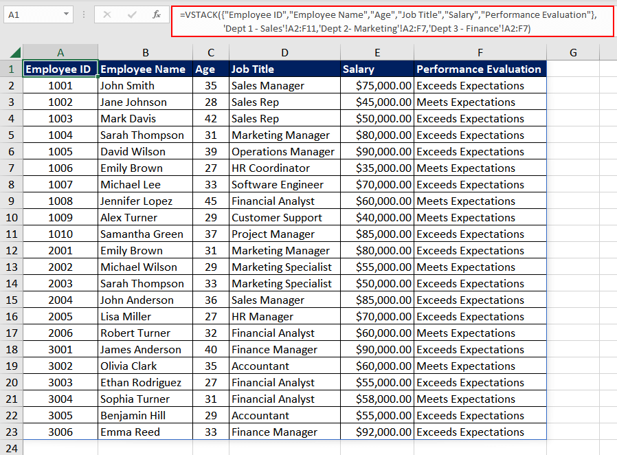
Now we have the required data in one sheet. In this case, we only had 3 sheets to combine, imagine if there were 20 of them. It would be inefficient to visit each sheet and select the cell range. Instead, we can use a dynamic way of selecting cell references, which is a 3D reference. It allows us to refer to cell ranges that span across multiple worksheets within a workbook.

Also, instead of selecting the cell range that contains the data, we will select a bigger cell range assuming data from each worksheet is covered within that range. The formula used will be as follows.

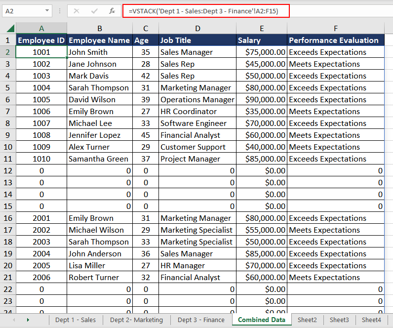
The formula merges the cell range A2:F15 from all the sheets starting from "Dept 1 – Sales' to 'Dept 3 – Finance'. Because the size of the dataset varies in each worksheet, the gap is filled with 0s. To remove that, we can use the FILTER function and include (TAKE Function) all the data which is not equal to 0. The formula used will be as follows.

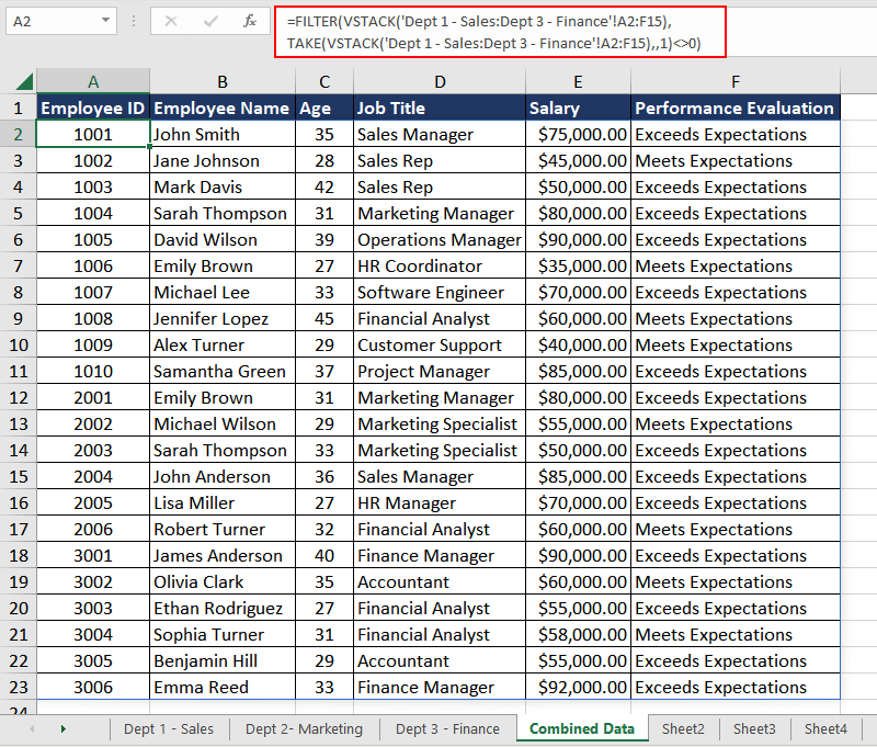
The best thing about this solution is that it includes any new sheet that is added between the 3D reference of the sheets, therefore creating a very dynamic solution to stack data.

VSTACK Function vs HSTACK Function

Now we know that the VSTACK function is used to vertically merge or stack cell ranges or arrays. On the other hand, the HSTACK function is used to horizontally append datasets. Both functions are used to selectively combine the data according to our needs, with the difference being that one operates in a column-wise manner, while the other operates in a row-wise manner.

Let's take a simple example to better understand the contrast.

Here we have taken two small cell ranges B1:B2 AND C1:C2. The intention is to combine both vertically and horizontally. The formula used will be as follows.

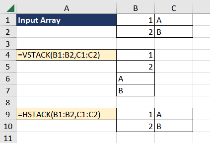
As required, the VSTACK function merged the two cell ranges while stacking them on top of each other. Conversely, the HSTACK function combines them horizontally, placing them side by side.

Practice and explore new applications to use the VSTACK function as it proves to be an excellent tool to clean data and is vastly used in data analysis. In the meantime, we will be back with yet another Excel function to expand your repertoire.