Check if a Value is in a List in Excel (9 Quick & Easy Ways)

Probable reasons you could be here today: confirming item availability, identifying whether a certain subcategory exists or not for data management, making decisions based on the presence of a value, extracting relevant information from large datasets, performing calculations conditionally, checking for partially matching text. Such important tasks to be carried out and aren't you glad paperwork is a thing of way yesterday?

Excel has so many means to check a list for a value, something is bound to fit the format of your dataset. We have easy mixes of functions to quickly cater to the mission and if you feel that they aren't as easy, all that is about to change; we have everything detailed in this tutorial.

Let's get evaluating!

Method #1 – Using Find and Replace Feature

Use the Find and Replace feature to check if a value is in a list in Excel. This feature is what Excel has in store for you when you press Ctrl + F on your worksheet. Find and Replace not only confirms whether a value is present on the worksheet, it also acts as a map and locator for the relevant cell.

Let's show you with an example of what this feature can do. Follow the steps below to check for a value in a list with Find and Replace:

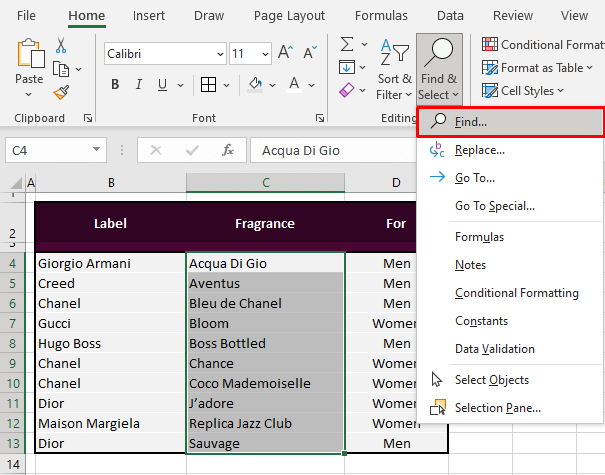
• Select the range where you specifically want to find the value. You may skip this step but since it's easy in our example case, we have selected the entries in the Fragrance column i.e. C4 to C13. You may select entire rows or columns or search the whole sheet.
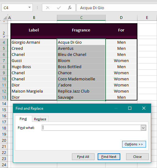
• Click on the Home tab's Find & Select button in the Editing Then select Find from the drop-down menu. Alternatively, use the Ctrl + F keys. Either way, you will be led to the Find and Replace dialog box.
• 
• The dialog box also shows an Options button which can help narrow down the search tunnel.
• 
• Type the value you want to search in the Find what
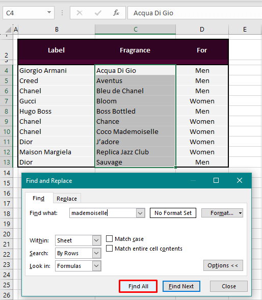
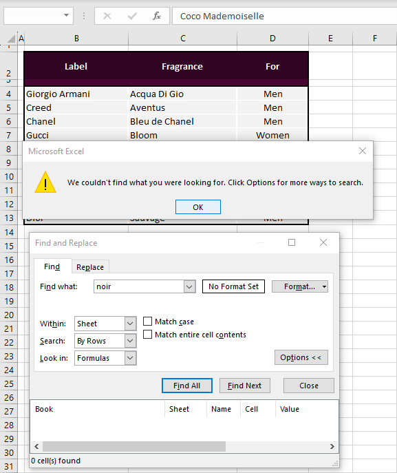
• E.g. we want to check for a fragrance called "Coco Mademoiselle". We have only searched using the word "mademoiselle".
• Hit the Find All

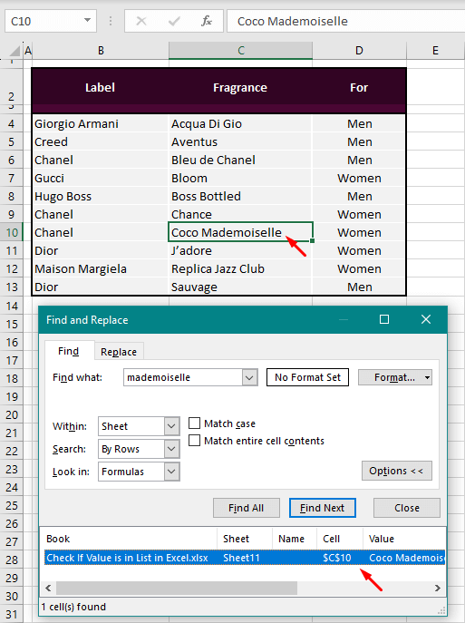
You will be navigated to the first cell in the selection with the provided value ("mademoiselle"). Find and Replace also shows the complete location details of the searched value and all the instances of that value in the selected cells.

If the searched value is not in the selected cells, an error message will pop up as shown below. This message was displayed after we tried searching for "Noir" in the fragrance column which is not listed.

Now you won't always have a widget hovering on your spreadsheet, reminding you of the status of availability so you might need to pen this information down. Why don't we get Excel to do that for us? Let's explore the many ways Excel jots the presence of a value down.

Method #2 – Using COUNTIF Function

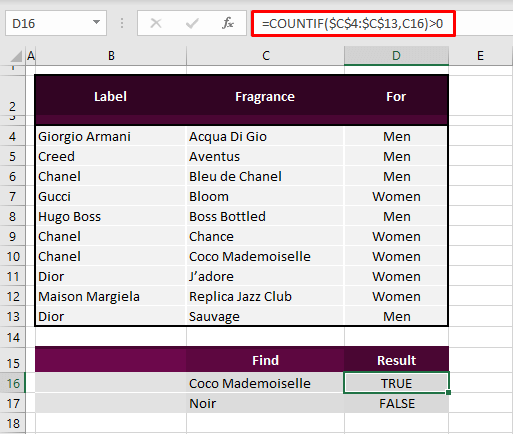
Check a specific value in a range using Excel's COUNTIF function. The COUNTIF function will count cells that fulfill set conditions. COUNTIF will count the cells with the search value and notify us if that count exceeds 0 or not. The formula as per our case example has been drafted as follows:

Give COUNTIF the range where it must search and count which is C4:C13 in this case. Then enter the search value. We have entered C16 as it contains the search value. We can also replace the cell reference C16 in the formula with "Coco Mademoiselle" enclosed in double quotes.

There is only one cell with the value "Coco Mademoiselle" so COUNTIF will return 1. Therefore, ">0" has been added to the formula to get the result in TRUE or FALSE. The formula boils down to 1 > 0 which will result in TRUE.

For the next search value "Noir", the count will be 0. 0 is not greater than 0 so the result is FALSE. If you are searching a single value, you don't need to lock the range as an absolute reference but since we are searching for 2 values here, when the formula will be copied down, the search range will also shift downward. To avoid that, C4:C13 has been locked with a dollar sign ($) in place.

COUNTIF with Custom Text

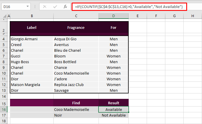
You can further tailor the formula to return custom results simply by enclosing the formula above in the IF function. See the formula below:

The COUNTIF function has been wrapped in the IF function with values provided for TRUE and FALSE results as "Available" and "Not Available" respectively.

You may have noted that in searching for a value this way, you need to be completely mindful of the value but that can't always be the case, right? Say, we don't remember the full name of the fragrance and only recall "Mademoiselle". If we try searching just this value, it will come up as unavailable because only cells containing just "Mademoiselle" will be searched.

COUNTIF with Partial Value

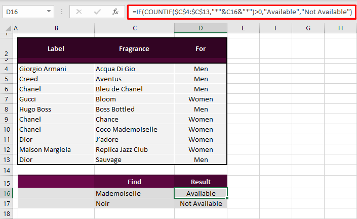
There is still hope for us. We can amend the formula with a wildcard operator (i.e. the asterisk *). Search cells for a partial value with the following formula:

The only difference we have now made is to the search value (the second argument in the COUNTIF function). The search value has been wrapped in the & operator to fix the wildcard operator on both sides. The wildcard operator itself is wrapped in double quotes.

This will serve as a wildcard and will search all values in the range with the word "Mademoiselle". Any words before and after "Mademoiselle" will be handled by the wildcard operators.

Method #3 – Using OR Function

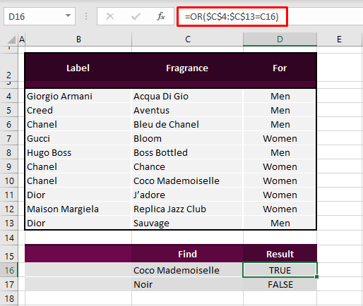
Check a list for a particular value with the OR function in Excel. The OR function returns FALSE only if all arguments are FALSE. For any TRUE argument, OR will return TRUE. We can set the OR function to check the search range for the search value. If even once the value is found, OR will return TRUE. If not, it'll result in FALSE. Fair deal and fairly simple. This is what the formula should look like:

We have added the search range in the formula so the OR function can check whether any cell in C4:C13 equals C16. In other words, if C4:C13 contains "Coco Mademoiselle". The OR function finds the value in C10 and hence returns TRUE.

Method #4 – Using SUMPRODUCT Function

The SUMPRODUCT function can be tweaked to check a list in Excel for a given value. SUMPRODUCT returns the sum of the products in a range.

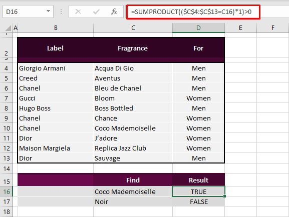
While that sounds off track, we can use some formats from the previous methods to get SUMPRODUCT to function in the direction of checking a value. Have a look at the formula ahead and the description to see how the SUMPRODUCT function identifies the presence of a value in a range:

The common bits we see here are the search range and value; C4:13 is being checked for C16. Multiply that by 1 as SUMPRODUCT's requirement to process a single condition (the condition being C4:13=C16). Up to this point, SUMPRODUCT will work like COUNTIF and return the number of cells matching C16. The 'greater than 0' addition will convert the count to TRUE or FALSE.

Method #5 – Using MATCH and ISNUMBER Functions

Use the MATCH and ISNUMBER functions to check if a value is in a list in Excel. The MATCH function checks an array for a matching value and returns the position of the matching cell in that array. Quite close to what we're looking for, is it not?

And by now you've probably figured that we can modify a formula to get TRUE/FALSE or custom text instead of numbers. Right you are. Proceed to the formula down here and witness the magic of the MATCH and ISNUMBER functions checking a range for a value:

The MATCH function takes the lookup value (C16) and lookup array (C4:C13). 0 is entered for returning an exact match. MATCH will search the array for the value and return 7 in this case since that is the position of "Coco Mademoiselle" in the search range.

If no match was found (e.g. "Noir" can't be found in the next instance), MATCH will return an error. Thus, ISNUMBER returns TRUE if MATCH results in a number, otherwise it returns FALSE.

Method #6 – Using XLOOKUP, ISERROR, and NOT Functions

A combination of the XLOOKUP, ISERROR, and NOT functions can help check a range for a value in Excel. The XLOOKUP function searches a range for a value and returns another corresponding value from a second range (used for horizontal and vertical lookup).

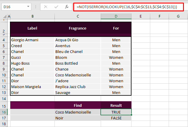
We can set the lookup range and second range as the same. The rest of the story is detailed following the formula below:

The XLOOKUP function searches C16 in C4:C13 and returns the same value from that range since we have set the lookup and second range, both as C4:C13. If the search value isn't found, XLOOKUP throws an #N/A error. ISERROR takes care of the #N/A error but would give us the opposite than desired results.

• Lookup value found > Error? > FALSE
• Lookup value not found > Error? > TRUE

So we'll have FALSE if the value is found and TRUE if it isn't. Let's reverse that with the NOT function and there we have the appropriate outcome; TRUE when found and FALSE when not found.

Method #7 – Using VLOOKUP, ISERROR, and NOT Functions

Check a specific value in a range using Excel's VLOOKUP, ISERROR, and NOT functions. And one may wonder what the point is of mentioning a near copy of the previous method with XLOOKUP swapped for VLOOKUP. XLOOKUP may have the ability to do it all but it's not an option for non-MS 365 and non-Excel 2021 users.

VLOOKUP will be used in the same manner as XLOOKUP as done in the previous method; it will search the value in a range and return the corresponding value which will then be passed to the ISERROR and NOT functions. The complete formula for checking a specific value with VLOOKUP is:

The VLOOKUP function will look for the value in C16 in the range C4:C13 and return the value from the first column in the given range (since we have only given one column in the range, VLOOKUP will return the value from the same column). For an exact match, the last argument is provided as FALSE.

And again, VLOOKUP will either return the search value from column C or an error which will be converted to FALSE or TRUE (respectively) by ISERROR. Finally, the NOT function flips FALSE to true and vice versa.

Method #8 – Using INDEX, MATCH, and ISERROR Functions

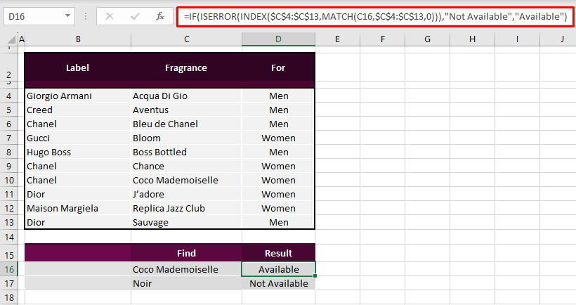
Combine the INDEX, MATCH, and ISERROR functions in Excel to verify if a list contains a value. The INDEX function returns the value at the intersection of a row and column. Using that aspect of the function, we can ascertain if a range contains a value or not. The grand mix of the INDEX, MATCH, and ISERROR functions can be found in the formula here:

The working range for the INDEX function is C4:C13. The row from where INDEX will return the value will be supplied by the MATCH function. The MATCH function will find an exact match of C16 in the range C4:C13 and return the row number of where the match value is. In the range C4:C13, the match value lies in row 7.

MATCH passes row 7 to INDEX which returns the value from row 7 as "Coco Mademoiselle". If the search value is missing from the range, there will be a resulting #N/A error. The ISERROR function changes found and missing values to FALSE and TRUE respectively.

From there, you can decide whether you want to place the NOT function or the IF function at the head of the formula. The NOT function will return TRUE or FALSE values while the IF function can return custom text. As an example, we've set the IF function to return "Not Available" in case of an error and "Available" for spotting the search value.

Method #9 – Using FILTER, ISERROR, and NOT Functions

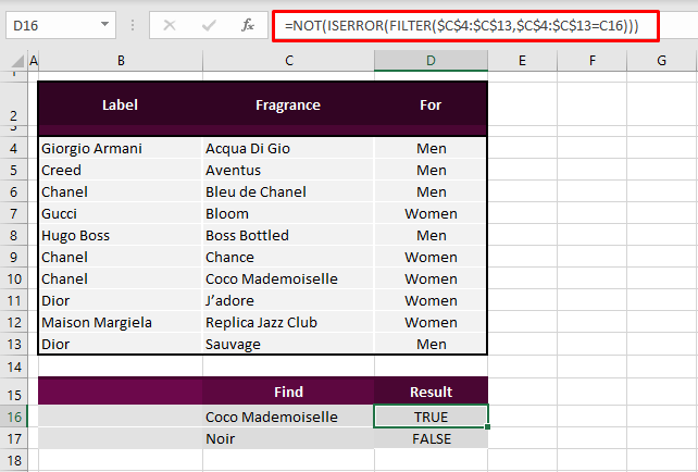
Check a list for a particular value with the FILTER, ISERROR, and NOT functions in Excel. The FILTER function filters a range. Our search value "Coco Mademoiselle" can be passed to the FILTER function and, if found, the value will be returned.

If not, it returns a #CALC! error. And then it's up to the ISERROR and NOT functions to handle what FILTER returns. A sample formula with these three functions is mentioned below:

First for the FILTER function comes the lookup array and then the text filter which is C16, given as Boolean (C4:C13=C16). FILTER returns the text filter value or an error that is converted to FALSE or TRUE by ISERROR and then switched by the NOT function.

We're ready to bet you have become a value-tracking alpha geek right about now but that only lays a scratch on the surface of the mighty iceberg that is Excel. We'll set you to make more grooves and dents and waves with valuable learning experiences. Ready? Tricky? Go!