You won't catch us trying to add only positive numbers from a list of mixed figures manually because Excel has more than one trick to get the job neatly done!
If you've run out of luck trying to switch and twitch your way around with the SUM function, we applaud you for your hard work and welcome you to this tutorial. Today you will learn how to add just one type of number using the SUMIF or SUBTOTAL function, an Excel Table, and VBA.
One of the only places where it's okay to be just negative. Let's go!

Method #1 – Using SUMIF Function
Sum just the positive or negative numbers using the SUMIF function in Excel. The SUMIF function adds cells that fulfill the given condition. We can set the condition in the function to sum all numbers greater than zero. Below we have an example that will show you how to use the SUMIF function for adding only positive numbers using the following formula:
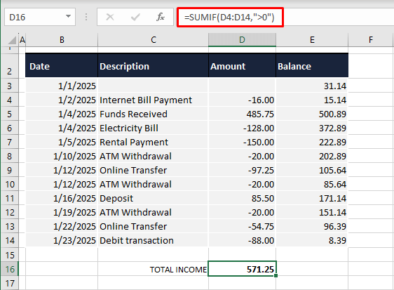
=SUMIF(D4:D14,">0")Column D in the example's dataset consists of a mix of positive and negative numbers representing inflow and outflow figures respectively. The SUMIF function is given the condition to add all numbers greater than 0 that are in the range D4:D14. These are the formula's results in the example:
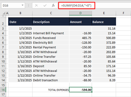
On the other hand, it is possible to use the same formula with a small change to calculate the sum of only the negative numbers. See below:
=SUMIF(D4:D14,"<0")We have changed the condition from greater than 0 to less than 0 in the formula and now we have the sum of all the negative numbers in column D:
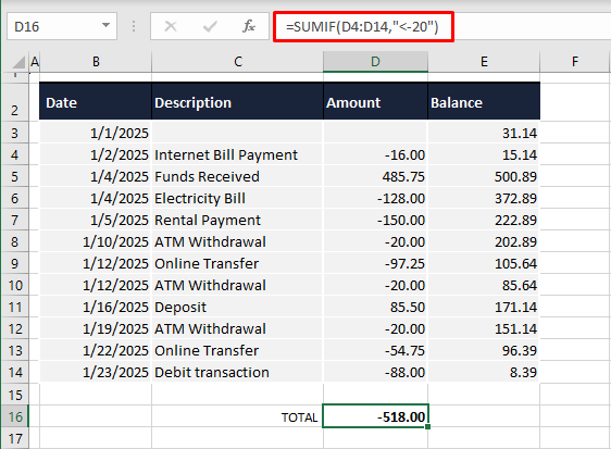
Rolling with the same concept, you can modify the condition to suit your objective. Let's say you aim to keep out some of the petty expenses from the summation, e.g. ones less than $20. You will then edit the formula to include the numbers greater than 20 but since in our example, the target values are negative, the condition will be the inclusion of numbers that are less than -20. The formula becomes:
=SUMIF(D4:D14,"<-20")This formula will then add all the expenses greater than $20 like so:
Showing Negative Numbers as Positive
You may have noticed in the last two instances that the output figure of our formulas is a negative number as a result of summing negative numbers. This might or might not be an issue but if it is a problem or a preference, the negative numbers can be changed to positive.
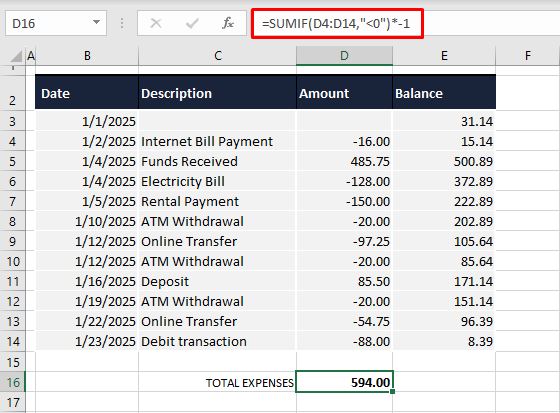
As shown in the earlier example, if we were using the SUMIF function for adding negative numbers, we can attach a small expression in the formula, multiplying it by -1. Here is the amended formula:
=SUMIF(D4:D14,"<0")*-1Multiplying the SUMIF formula by -1 ensures that the negative output is converted to a positive number. The SUMIF formula returns -594 and the amended formula becomes -594 * -1 which equals 594.
While the -1 multiplication is a master stroke and all, you may not always be using a formula that you can amend. For those cases, you can opt to format the formula cell so that it displays the negative value as a positive one.
If you are going with the formatting suggestion, select the formula cell (D16 here) and press the Ctrl + 1 keys to open the Format Cells dialog box. Go to the Number tab's Custom category and you will see the formatting code for the current format of the selected cell. This is what ours shows:
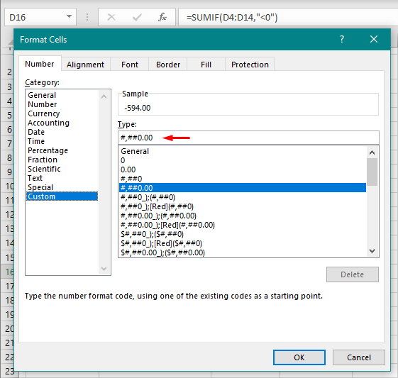
This is a formatting code for displaying numbers with two decimal places and a thousand separator. Our next format will display both positive and negative numbers as positive values. Enter the below-mentioned format in the dialog box's Type field:
0.00;0.00This code will ensure that both positive and negative values appear as positive numbers with 2 decimal places.
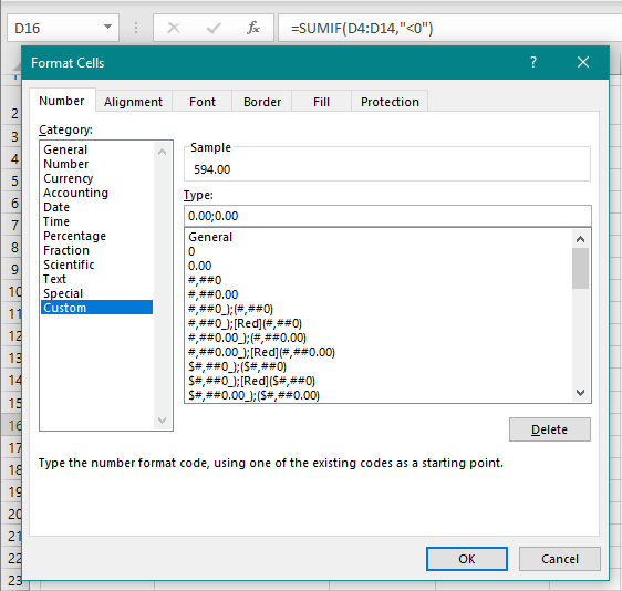
Click on the OK.
Now we have our final value in a positive appearance:
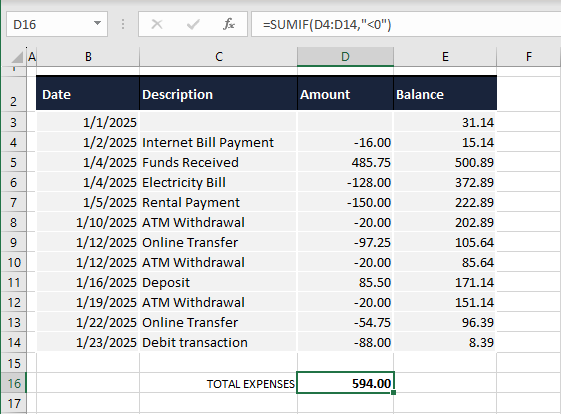
Changing the format will not change the actual negative value of the number, only the display. For more on changing negative numbers to positive, head here.
Method #2 – Using Excel Table Feature
Use the Excel Table feature to sum only positive or negative numbers. An Excel Table helps sort and analyze data easily and efficiently. We aim to employ the filter and Total Row feature for adding positive or negative numbers.
The filter will show numbers belonging to only one sign and the Total Row can sum the displayed numbers. The steps ahead will guide you on how to utilize an Excel Table to filter out the same sign numbers and sum them and we begin with converting our dataset to an Excel Table.
- Select any cell from the dataset that you want as a Table.
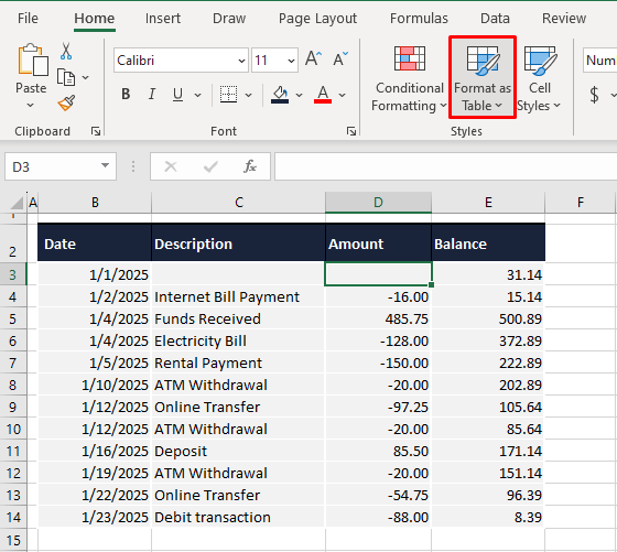
- In the Home tab's Styles group, select the Format as Table
- Click on a Table Style of preference from the menu.
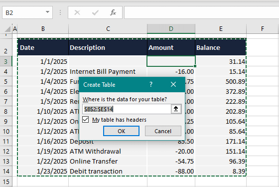
- Once a Table Style is selected, a small dialog box will pop up as the Excel Table feature tries to guess the range for creating the Table. A marching-ants line will encase the dataset that surrounds the selected cell, and the range will show up in the dialog box. Adjust if needed.
- Since our table has headers, we have left the checkbox in the dialog box marked.
- Hit the OK
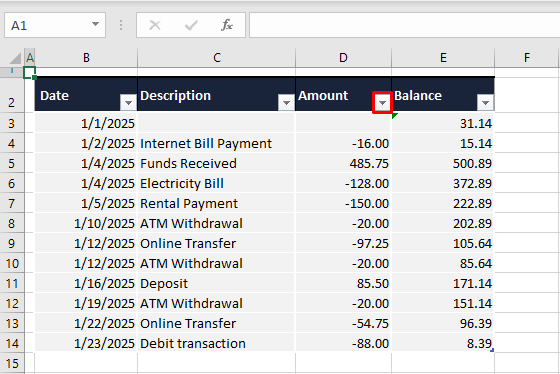
- The selected range will become an Excel Table and you will now see filters for every column in the Table.
- Click on the filter of the column that you want to sum the numbers from. In this example case, we are going to use the filter on the Amount
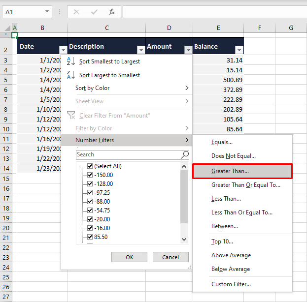
- Point to Number Filters in the menu and select the Greater Than option in the submenu.
- The Greater Than option will be used for the summation of positive numbers and The Less Than option for negative numbers.
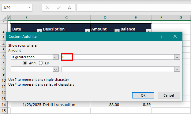
- In the Custom Autofilter dialog box, type 0 in the first text box (as highlighted below) so that the custom filter is set to "greater than 0".
- Click on the OK
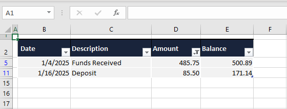
- All the positive numbers in the Amount column will only be displayed now.
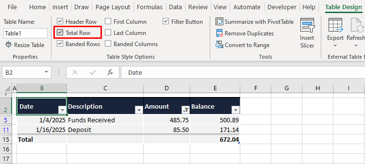
- Again, select any cell in the Table. This activates the Table Design Now click on the Table Design tab and select the Total Row checkbox from the Table Style Options.
- The Total Row will be added at the base of the Table automatically with the sum of the last numerical column in the Table. Since we are looking for the sum of the Amount column, we'll have to add it ourselves.
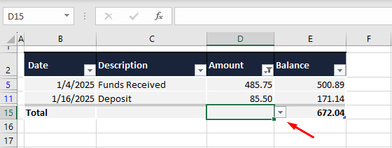
- Click on the cell where you want the total figure (D15 in the case example).
- A small, boxed arrow will appear with the cell.
- Select the arrow to open a drop menu and click on the Sum
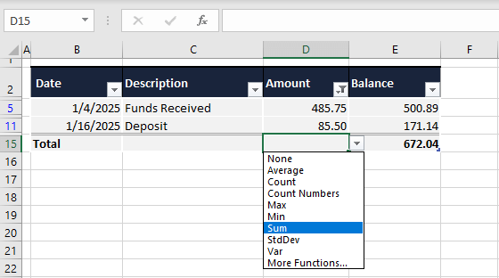
The sum for the Amount column will also show in the Total Row.
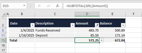
For filtering the negative numbers to sum them, apply the Less Than number filter.
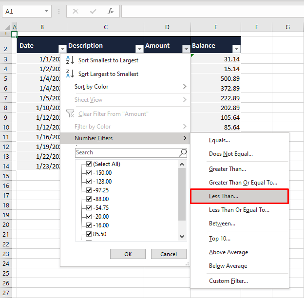
Confirm the amount as 0 in the Custom Autofilter dialog box, set the Total Row, and arrange the sum for the chosen column. You should be able to see the total for the negative numbers in the Total Row.
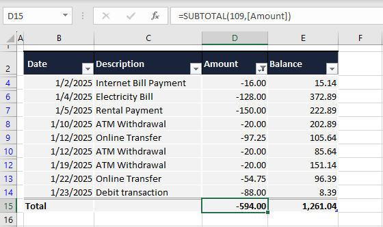
Notice how the Excel Table automatically applies the SUBTOTAL function for the sum? You'll see why shortly; proceed to the next section.
Method #3 – Using SUBTOTAL Function with Filters
Add just the positive or negative values from a set of numbers with Filters and the SUBTOTAL function in Excel. While a Table's Total Row makes quick work of summation, you do not need to set up an Excel Table to conveniently calculate sums. You can choose to apply the SUBTOTAL function directly with Filters.
The SUBTOTAL function returns a subtotal of a set of data based on the chosen function (e.g. SUM, AVERAGE, COUNT function, etc.). This section will also show you why the simple SUM function can't be of help in filtered data. Use the steps below to sum positive or negative numbers with the SUBTOTAL function and Filters:
- Select any cell in the dataset.
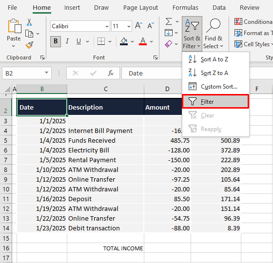
- Go to the Home tab > Editing group > Sort & Filter button > Filter
- The Filters can also be applied using a keyboard shortcut: Ctrl + Shift + L
- Once the Filters are on, you can use them on the relevant column to get the same sign numbers summed.
- Select the filter arrow of the target column (in this example, it's the Amount column).
- Hover the cursor on the Number Filters option and select the Greater Than or Less Than option for adding positive or negative numbers respectively.
- Add the value in the upcoming dialog box. We're adding 0.
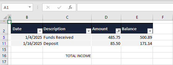
Here's the dataset filtered based on positive numbers in the Amount column:
Now as per a very general Excel understanding, if we are to add the figures in column D, the SUM function would be fitting?
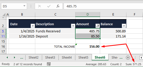
We can immediately tell that the SUM function hasn't performed as we wanted it to as it includes all the numbers from D5 to D11, even the ones bunched up in the filtered rows. Besides, if we select cells D5 and D11, the sum displayed in the Status Bar doesn't match the one produced by the SUM function. Therefore, we'll go with the SUBTOTAL function.
- Select the target cell for the sum (i.e. D16 here) and press the Alt + = keys to enter the SUBTOTAL function.
The first argument will automatically appear as number 9 which is the function number for the SUM function within SUBTOTAL. The function will also guess the list above the target cell as the range for the subtotal calculation.
- Adjust the range in the formula if required. Then hit the Enter key to apply the function.
The SUBTOTAL function will be entered with the SUM operative, adding only the displayed numbers in the selected range and not the hidden/filtered ones.
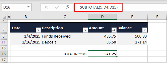
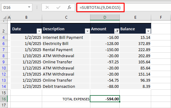
Similar steps can be performed using the SUBTOTAL function to sum negative numbers. As seen earlier, apply the Less Than 0 filter and enter the SUBTOTAL function for the summation.
Method #4 – Using VBA
VBA in Excel can be programmed to get the total of only positive or negative numbers. VBA is a programming language for Office that carries out tasks and adds functionality to Excel. Using VBA code, we will instruct the document to perform an addition calculation of same-sign numbers in the selected range.
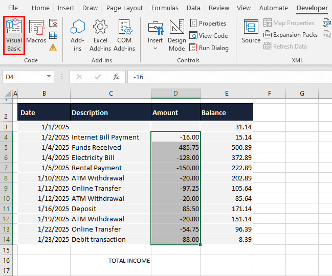
- Select the range with the numbers (D4 to D14 in the case example).
- Use the Developer tab to access the Visual Basic button in the Code If your Excel is lacking the Developer tab, you can enable it from the Ribbon settings or use the keyboard shortcut by pressing the Alt + F11 keys.
- Either method will launch the Visual Basic editor.
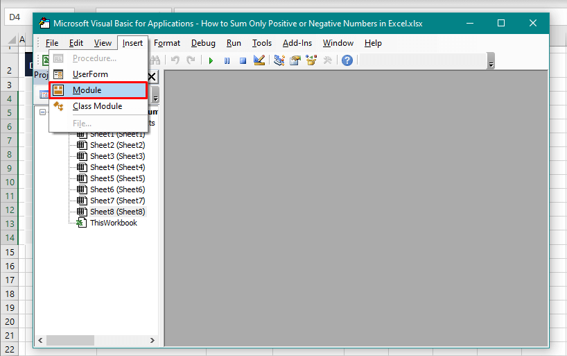
- In the editor, click on the Insert tab and select the Module option from the drop menu.
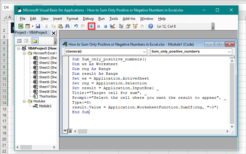
- Copy the code from here to the Module
Sub Sum_only_positive_numbers()
Dim ws As Worksheet
Dim rng As Range
Dim result As Range
Set ws = Application.ActiveSheet
Set rng = Application.Selection
Set result = Application.InputBox( _
 Title:="Target cell for sum", _
 Prompt:="Select the cell where you want the result to appear", _
 Type:=8)
result.Value = Application.WorksheetFunction.SumIf(rng, ">0")
End Sub
The second last line in the code dictates the values that are to be considered for summation i.e. ">0". Only the numbers greater than 0 will be added and this can be changed to "<0" for adding negative numbers.
- After pasting (and tweaking, if necessary), select the Run button in the toolbar or use the F5 key to run the code.
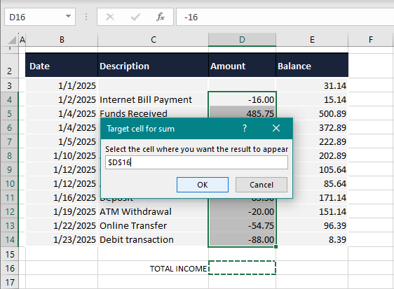
- An input box will appear.
- Click on the target cell (D16 for us) from the worksheet or enter the cell address in the box. Then hit OK.
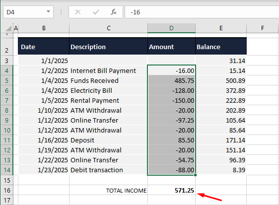
The summation figure will be displayed in the target cell.
And for the negative numbers, change the code as mentioned above or directly use the code given below:
Sub Sum_only_negative_numbers()
Dim ws As Worksheet
Dim rng As Range
Dim result As Range
Set ws = Application.ActiveSheet
Set rng = Application.Selection
Set result = Application.InputBox( _
 Title:="Target cell for sum", _
 Prompt:="Select the cell where you want the result to appear", _
 Type:=8)
result.Value = Application.WorksheetFunction.SumIf(rng, "<0")
End Sub
The only things we have changed in the code are the condition to less than zero "<0" and the title of the code. The sum will arrive as promised:

Can we assume that adding up numbers belonging to the same sign won't pose problems now? We're counting on you to deal with this task like a boss. For more boss moments, keep dropping by our Excel tricks and tips. Ready? Tricky? Go!
 Now as per a very general Excel understanding, if we are to add the figures in column D, the SUM function would be fitting?
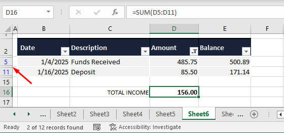 We can immediately tell that the SUM function hasn't performed as we wanted it to as it includes all the numbers from D5 to D11, even the ones bunched up in the filtered rows. Besides, if we select cells D5 and D11, the sum displayed in the Status Bar doesn't match the one produced by the SUM function. Therefore, we'll go with the SUBTOTAL function.
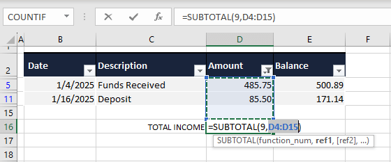 The first argument will automatically appear as number 9 which is the function number for the SUM function within SUBTOTAL. The function will also guess the list above the target cell as the range for the subtotal calculation.