How to Change Conditional Formatting in Excel (Step-by-Step)

The world is ever-changing and the Excel universe can say the same. With changes in data, requirements, users (and even moods?), there may need to be a change in what bits of the dataset are made prominent or how.

Changing from top 10 to top 5, from Data Bars to simple highlighting, from top 3 to the 90% percentile, highlighting cells with an added condition in the formula, from red cells to orange cells – these are some examples of why you would want to change the way Conditional Formatting is working.

A Conditional Formatting rule is used to format a range according to certain conditions. A created rule can be edited any time to change the rule's type, description, format, or the range that it applies to. Our tutorial is about changing Conditional Formatting in Excel which refers to changing the formatting rule.

Let's have a change of Excel scenery!

Recommended Reading : All You Need to Know About Conditional Formatting In Excel

Changing Conditional Formatting Rule

First things first, the one way to change a Conditional Formatting rule is by using the Rules Manager to edit the rule. The Rules Manager is accessed from the Manage Rules option in the Conditional Formatting menu.

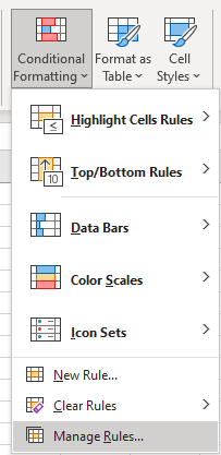
Don't be tempted to attempt overwriting a rule using the listed rules in the menu. This will not edit an existing rule but will create a new rule. In some cases, the new rule may overlap the old rule where the new rule covers more cells and so, on the face of the worksheet, it would appear that there is only one rule. But take into consideration that if the file is to be shared, anyone who would look into the Conditional Formatting might be confused by overlapping rules.

To save anyone or your later self from that time-wasting puzzlement, edit a rule instead of adding another one.

You may find it easier to edit a rule where the rule type, formatting, target range, or formula applied in the rule is the same in the existing and intended new rule. However, that may not always be the case. If the existing rule is far off from being edited conveniently and where it would prove quicker to add another rule, delete the previous rule so you can enter a new one.

Today's tutorial assumes that changing the Conditional Formatting rule is going to be the better option. By the time we are done, you will learn how to edit a rule by changing the rule type, rule formula, and rule formatting.

Changing Rule Type

A Conditional Formatting rule can be changed by changing the type of the rule. Changing the rule type alters the rule description parameters and this method of editing is most convenient where the rule has the covered range or the formatting in common with what you want to change the rule into.

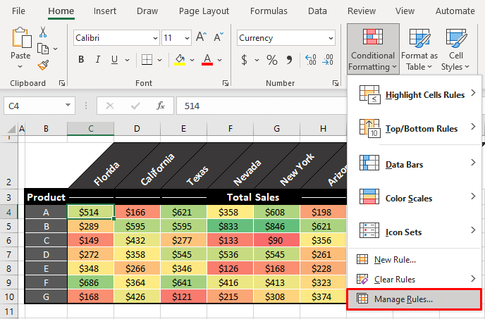
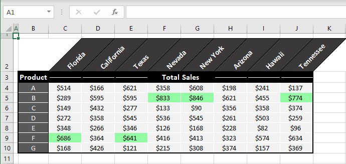
Let's investigate an example. The sample dataset below is made up of sales figures categorized by state and product. The sales values have been highlighted using a 3-Color Scale in Conditional Formatting creating a heatmap.

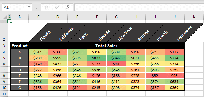
While a Color Scale does well to indicate the rank of each cell against the whole range, if we want to focus on the top 5 cash cow points, from a quick analysis point of view, it would be better to have just the top chosen number of figures highlighted.

We'll attempt to transform this fully highlighted dataset into just highlighting the top 5 values since we want to apply the top 5 rule to the same range. See the following steps for changing the type of a Conditional Formatting rule in Excel:

• Select any cell in the dataset that is covered by the Conditional Formatting. (You can also view all the rules in the worksheet in the Rules Manager later.)
• From the Home tab, first select the Conditional Formatting icon in the Styles group and then select Manage Rules from the options.
• 
• This option leads to the Conditional Formatting Rules Manager which displays all the formatting rules for the selected option in Show formatting rules for, located at the top of the Rules Manager.
• Click on the rule you want to edit and then select the Edit Rule

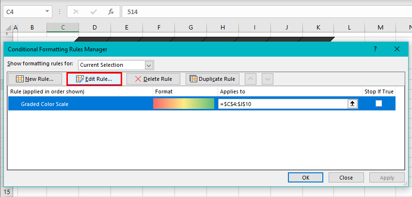
Tip: By default, the Rules Manager always shows the rules for the current selection. You can get the Rules Manager to display the rules for the entire worksheet by selecting This Worksheet in the Show formatting rules for bar. You may find this option particularly helpful if the manager doesn't display the rule you are looking for under the current selection.

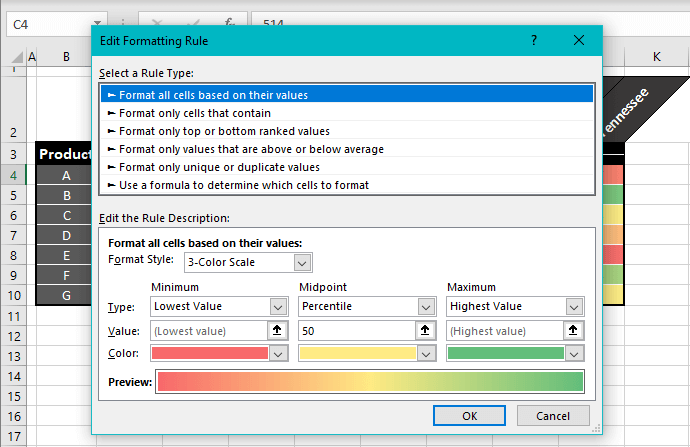
• A dialog box will open for editing the rule. Right now, the Edit Formatting Rule dialog box displays the particulars regarding the rule as we can see the details for our 3-Color Scale rule:
• 
• Change the rule type from the Select a Rule Type section, along with any other details that need changing.
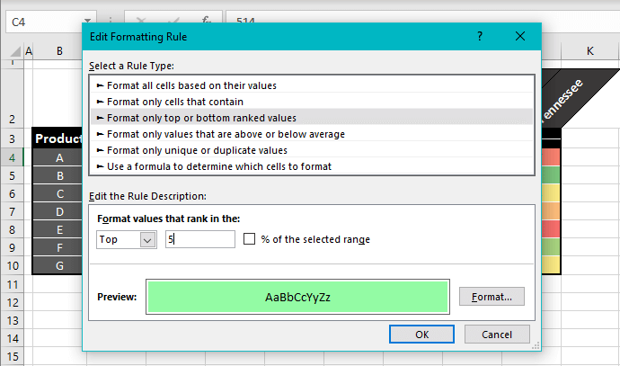
• In this example case, we are changing the rule type from Format all cells based on their values to Format only top or bottom ranked values. For the top 5, we have set the value in the text box to 5 and have selected a green color fill for the top 5 highlighted cells.
• 
• After the changes, hit the OK
• The dialog box will be closed and the changes to the rule will be reflected in the Rules Manager.
• Tip: As a time-saver, you can use the Apply button in the Rules Manager to see if the rule has worked on the sheet as you had expected. So that if it hasn't, the Rules Manager will be open for you to quickly edit the rule again.
• When done with the manager, select the OK

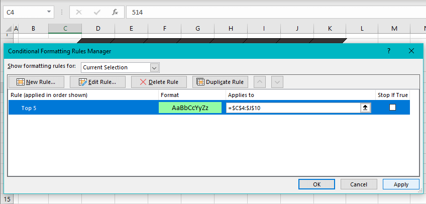
The rule has been changed and the Color Scale has been replaced with the highlighted top 5 values for the same range:

Changing Rule Formula

A Conditional Formatting rule can also be changed by changing its underlying formula. A formula is used in a rule usually when the other preset rules don't carry the type of condition you want to apply. If the rule formula needs a small change or needs a complete change while being used for the same range or formatting, then there makes little sense to apply a new rule instead of editing the ready one. The steps ahead will show you how to change a rule's formula in Excel.

Explaining this with an example, we have highlighted the participants under the age of 40 who took over 10 hours to complete test exercises.

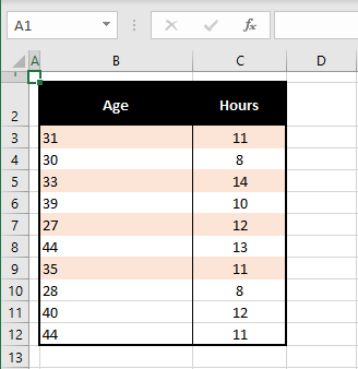
With some recalculations, the average time taken for the completion has changed slightly and we now aim to highlight participants under 40 years taking longer than 11 hours. Here's what to do.

• Select a cell containing the Conditional Formatting
• Open the Rules Manager from the Home tab > Styles group > Conditional Formatting icon > Manage Rules
• Click on the rule you want to edit and select the Edit Rule

Below is the description of the current rule without the changes. The formula used is:

For highlighting under 40 years and over 10 hours.

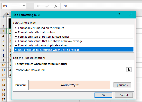
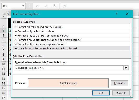
We are going to change just the 10 in the formula to 11 to highlight over 11 hours in the dataset. The formula now becomes

• Make the preferred changes to the formula in the given text box.
• 
• Select OK on the dialog box and the Rules Manager after editing and confirming the rule.

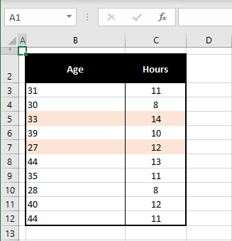
The changes in the rule formula have turned out just as well as it has highlighted the participants who took longer than 11 hours and are under 40:

Changing the Formatting

One way is to change the very look of the rule and that is done by changing the formatting. The formatting is also changed by editing the rule and you can follow the example below to do so.

Can you even tell what is happening in this example?

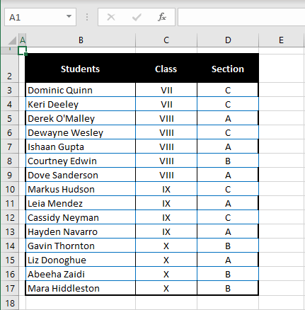
You might have picked out that there is an alternate thing going on (or trying to go on). The problem here is that we wanted every alternate row selected but the formatting has been set to blue borders for the selection. This is not immediately clear upon viewing the list and there's no need to adhere to the ambiguity when there are better options.

We can keep the formula while changing the format applied for the selected rows and we'll demonstrate how to do that with these steps:

• Select a cell from the Conditional Formatting
• Launch the Rules Manager from the Manage Rules options in the Conditional Formatting
• Select the relevant rule in the manager and hit the Edit Rule
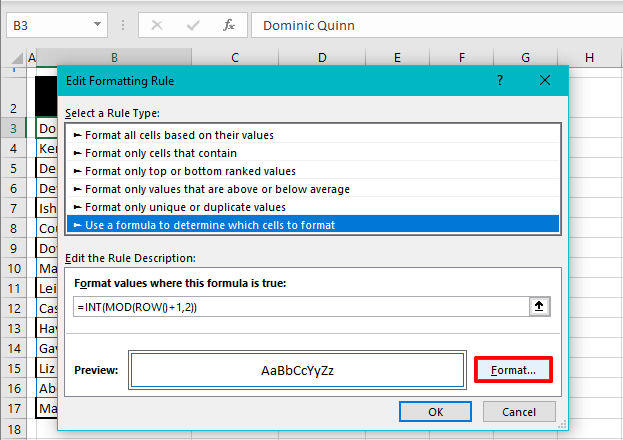
• Details of the current rule will open:
• 
• The format is set to blue borders with no fill.
• Click on the Format button highlighted above to change the format.
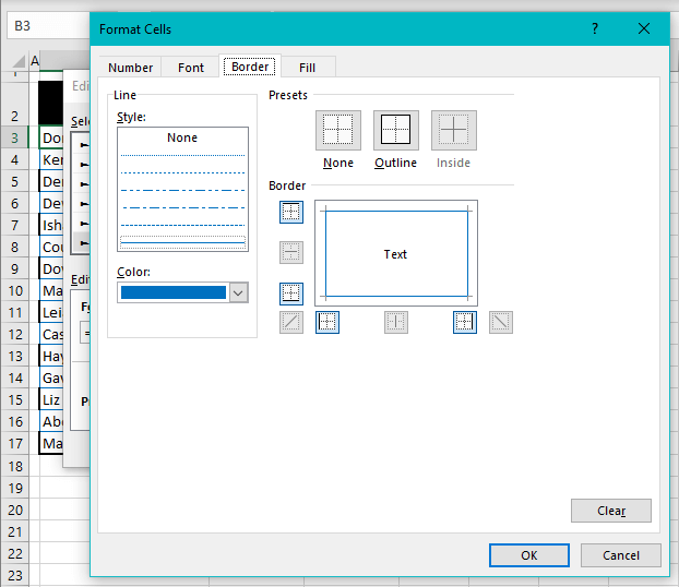
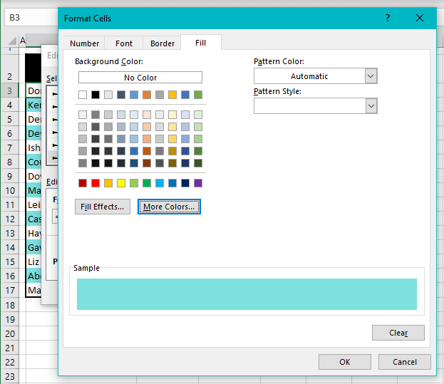
• We'll swap out the hollow border look for plain color fill using the Border and Fill tabs in the Format Cells dialog box to make the changes.
• 
• Set the color of choice for the highlighted cells and click on OK when done.
• 
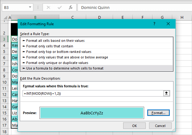
• The format change will show in the Edit Formatting Rule dialog box:
• 
• Use the OK command here and in the Rules Manager when the editing is done.

Behold the stark contrast of the changed format:

That saves straining our eyes.

You can take any Conditional Formatting rule, turn it on its head and change it into what you require and now you know well about how to accomplish that. We hope to have made a good job of showing you how easy the whole drill is. There will be more simplifying of Excel aspects coming up. No matter how tricky, we'll have a few Excel tricks ready for it!