Excel ARRAYTOTEXT Function – How To Use

The ARRAYTOTEXT function is used to convert any range of values into a single text string. The function simply combines the data from an array of cells into a single cell resulting in one text value or array. Depending on the format, the ARRAYTOTEXT function separates the data using either commas (,) or semicolons (;).

The ARRAYTOTEXT function is very useful when a large amount of data is to be processed further in text or array format.

Syntax

The syntax of the ARRAYTOTEXT function is as follows.

Arguments:

The ARRAYTOTEXT function accepts two arguments, and the usage of each is described below.

'array' – This is a mandatory argument that accepts the array of values that is to be transformed into a single text or array.

'format' – This is an optional argument that only accepts boolean input of 0 or 1. The default value of the format argument is 0, which translates to a concise format.

The concise format returns the data in a single cell combined using commas (,). When the value of the format argument is set to 1, the resulting data is in the strict format where each value is wrapped in double quotes, and the entire return value is in the form of an array with curly braces.

Important Characteristics of the ARRAYTOTEXT Function

Some of the noteworthy attributes of the ARRAYTOTEXT function are given below to provide a more comprehensive understanding of the function.

• If the data in the input array contains any number formatting, the ARRAYTOTEXT function removes the formatting in the return value.
• When the value of the format argument is 1, in the resulting text array, the data from rows are combined by semicolon (;), and column data is combined with a comma (,).
• If the input array contains booleans, numbers, or errors, and the value of the format argument is 1, the ARRAYTOTEXT function does not add double quotes to such values.
• If the value of the format argument is anything except 0 and 1, the ARRAYTOTEXT function throws a #VALUE! error.
• The return value of the ARRAYTOTEXT function when the format is set to strict can be directly used in formulas that accept text arrays.

Examples of ARRAYTOTEXT Function

Now that we have a basic overview of the ARRAYTOTEXT function let's understand different ways and applications where we can use the function.

Example 1 – Simple Use of ARRAYTOTEXT Function

Here we have taken sample data to better understand the primary nature of the ARRAYTOTEXT function.

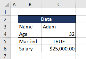
We will set the value of the format argument to both 0 and 1 to understand the contrast better with the same input values for the array argument.

In the first example, we are taking the values in column B as the input array, and all data is in text format. When the value of the format argument is set to 0, the function combines all the data with a comma and returns one text value in cell F3. On the contrary in the next case, when the format value is 1, it returns a text array with curly brackets where each value is encapsulated in double quotes separated by a semicolon.

In the third example, the input array contains the data from column C which includes a text, number, boolean, and a currency value. In the concise mode, all the values are combined with a comma commas, and the currency data loses its formatting. The concise format simply converts all the values into a text format and combines them.

In next instance in the strict mode, the text value is wrapped in double quotes while the numerical and boolean value stays as it is. The currency data, in this case, loses its formatting too. The remaining formatting stays the same in curly brackets separated by semicolons.

In the final example, the complete array from B3 to C6 is used as an input value for the array argument.  The values are treated in a similar fashion as the examples above. An additional thing to note here is that values from columns are combined using a comma, such as  "Name" and "Adam" from cells B3 and C3, whereas data from rows are separated using a semicolon like "Adam" and "Age" from cells C3 and B4.

Now the simple use of the ARRAYTOTEXT function is clear, let's explore some interesting examples, making more complex use of the function.

Example 2 – Combining Emails to Send Bulk Emails

In this example, we have received a list of subscribers with their email IDs for our latest newsletter. We now wish to combine all the email IDs in a single cell to be able to send the newsletter at once. Depending on the mail program to be used, all the emails can be combined using a comma or a semicolon.

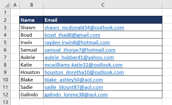
Here, we are using Gmail to send out all the emails, therefore, we can combine the email IDs using a comma. With the help of the ARRAYTOTEXT function, the formula used will be as follows.

We are using the default value of the format argument, which is 0, as we just want the data to be combined in the same format using a comma. The same result can also be achieved using the TEXTJOIN function.

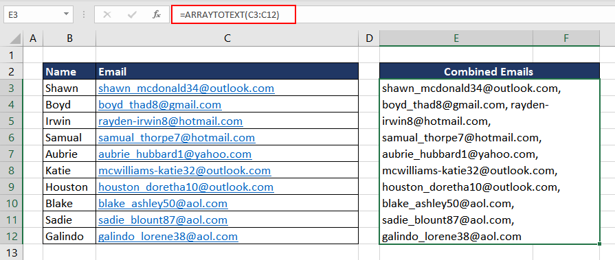
Now, we can directly use the resulting data from cell B15 in the email provider and send out the newsletters.

Example 3 – Combining Unique Data with ARRAYTOTEXT Function

In this scenario, we organized an online conference and based on the attendees, we wish to determine what kind of professionals participated and from which countries. Here we have a list of names along with their professions and countries.

As there is repetitive data, we can use the UNIQUE function to extract the different countries and professions. To collate the data in one cell, we will use the ARRAYTOTEXT function to combine it in one cell. The formula used will be as follows, one for countries and another for professions.

Here we are using the 'strict' option of the ARRAYTOTEXT function by assigning 1 to the format argument as we want to use the data for further processing.

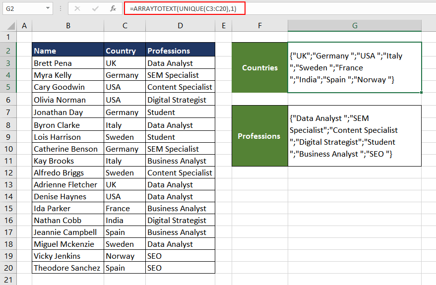
The countries and professions have been returned separated by semicolons, each enclosed in double quotes.

Example 4 – Autofill Numbers with ARRAYTOTEXT Function

There are instances when we require a simple sequence of numbers. One of the ways to do so is by using the SEQUENCE function and spilling the numbers into rows or columns as required. But, if we want the numbers in one cell, we can use the combination of SEQUENCE and ARRAYTOTEXT functions to get the desired sequence.

Let's create a series of numbers 1-15 in a single cell. First, let's use the SEQUENCE function to create a simple series in rows. The formula used will be as follows.

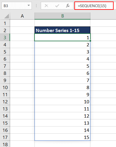
Now that we have the series in rows, we can use the ARRAYTOTEXT function to combine the data in a single cell. The function used will be as follows.

Depending on where the resulting data is to be used, the value of the format argument can be changed.

Now you know how to generate any series of numbers in a cell just in one step. Using the same logic, we can also have an alphabetical series in a single cell.

Example 5 – Autofill Alphabets with ARRAYTOTEXT Function

For instance, we need all the alphabets from A to Z in a single cell. You can either choose to manually write each letter and combine them with a comma or use the above logic with slight improvements to get the desired result.

We will combine CODE, CHAR, SEQUENCE, and ARRAYTOTEXT functions to generate and autofill letters A to Z in a single cell. Let's understand the role of each function.

The CODE function will first return the Unicode of the letter 'A', which is 65. We will then attempt to create a sequence of numbers starting from the Unicode of the letter 'A' for up to 26 rows, as there are 26 letters in the English alphabet. Then we wrap the return result in the CHAR function, which will give us the characters corresponding to each Unicode, eventually translating to uppercase letters A to Z.

Let's translate that logic into Excel functions. The first step is to create a sequence of Unicode ranging from 65 to 90. The formula used will be as follows.

This formula will create a sequence of numbers in 26 rows starting from the Unicode value of the uppercase letter A and up to Z.

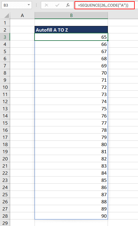
Now that we have the series of Unicode, we wrap the formula in the CHAR function. The updated formula will be as follows.

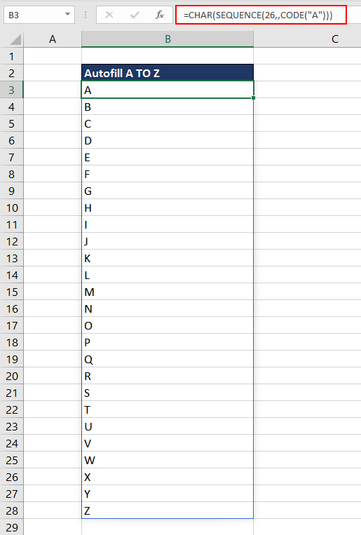
We will now use the ARRAYTOTEXT function to combine all values from the rows in a single cell. The final formula will be as follows.

Easy enough, right? Now you can easily add any number of alphabets in a single cell using the above function.

Hopefully, you enjoyed learning the ARRAYTOTEXT function and the different ways to use it. Practice the same and discover new applications of ARRAYTOTEXT while we come up with our next Excel function.