Excel TEXTSPLIT Function – How To Use

The TEXTSPLIT function separates the input text into columns and/or rows as per the given delimiter. The resulting text is spilled into different columns and rows, creating an array. It is one of the most useful Excel functions for text structuring and editing.

The TEXTSPLIT function is like the in-built Text to Columns functionality of Excel, where the text is split as per width or delimiter. The results of the TEXTSPLIT function will be dynamic whereas the ones from Text to Columns will not.

Syntax

The syntax of the TEXTSPLIT function is as follows.

Arguments:

There are several arguments in the TEXTSPLIT function, out of which only two are mandatory.

'text' – This is a mandatory argument and accepts the value of the input text we wish to split. It can be a direct value in double quotes or a cell reference containing the text.

'col_delimiter' – This is also a required argument which is the text, space, or character that divides the text to be separated in columns. The value of the col_delimiter is where the text is split and spilled into columns.

'row_delimiter' – This is an optional argument and accepts the value of the text, space, or character that marks the separator from where the input text can be split into rows.

For both col_delimiter and row_delimiter, the value can be passed as an array in curly brackets if more than one delimiter is to be used.

'ignore_empty' – This is an optional argument that only accepts TRUE or FALSE as input values. Alternatively, we can also use 1 and 0, respectively. As the name suggests, this argument instructs the TEXTSPLIT function to ignore or include empty cells. The default value of ignore_empty is FALSE, which includes the empty cell and creates one in the result if a value is missing or consecutive delimiters are in the text. If the value is set to TRUE or 1, the function ignores the consecutive delimiters.

'match_mode' – This is an optional argument and accepts Boolean input values – 1 or 0. The default value of match_mode is 0, which makes the function case-sensitive. If the value is set to 1, the TEXTSPLIT function performs a case-insensitive match.

'pad_with' – This last argument is also an optional one. The default value of the argument is #N/A. If a value is missing in a resulting 2D array, the empty cell is padded with the input value of this argument.

Important Characteristics of the TEXTSPLIT Function

One of the most basic characteristics of the TEXTSPLIT function is that as it is a text category function, the resulting values are always in the text format. Other noteworthy features of the function are as follows.

• The TEXTSPLIT function returns a #VALUE! error if the input value of the text is left blank.
• At least one delimiter argument must be used, else the TEXTSPLIT function returns a #VALUE! error.
• If the resulting text or array doesn't have enough space to spill, Excel returns a #SPILL! error.
•  When the value of the match_mode argument is set to 1, the resulting text is always in lowercase.

Examples of TEXTSPLIT Function

As the TEXTSPLIT function contains several arguments, it's important to make sense of the usage of each for a comprehensive understanding of the function. Below mentioned are numerous examples explaining each of the arguments.

Example 1 – Basic Functionality of TEXTSPLIT Function

Here, we are taking different data sets to understand different ways to use the TEXTSPLIT function.

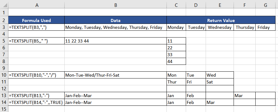
In the first example, the days of the week are separated using a comma in the input text in cell B3. Using the comma as the col_delimiter, we will segregate the input text into separate columns. The result is as expected from cell C3 to G3.

In the next example, we are trying to split the input text into different rows. So, in this case, we will use the separator as a row_delimiter and leave the col_delimiter empty as seen from cells C5 to C8. It can also be noted that even if the input text were numbers, the return value is in the text format, which is evident due to its left alignment.

So, till now, we are clear about how to split the text into columns and rows separately. In the next example, we will try to split the text into both, creating a 2D array. We will use one separator as col_delimiter, a dash in this case, and the other one as row_delimiter, which is a forward slash. The return value is as expected, as seen in cell range C10:E11.

The next two examples demonstrate the use of the argument ignore_empty. As we know that if no value is assigned, the default value is FALSE, which includes the empty cell in the result of the 4th example. In the fourth example, we are trying to split the month names, separated by a dash. Cell E13 is empty as data is missing in the input text.

In the next example, we include the value of the ignore_empty argument as TRUE, and there is no empty cell as the function ignores consecutive delimiters or missing data. The use of the other two arguments will be clear in the further examples.

Example 1.1 – Splitting Data into Columns using TEXTSPLIT Function

In this example, we have the names of top Olympic athletes, the country they represent, and the sport. For better understanding, we wish to divide the text into separate columns.

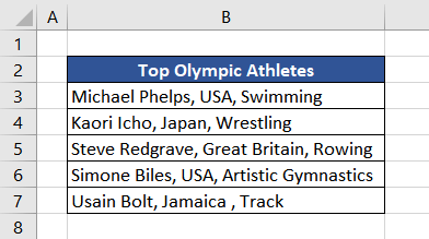
We can see that each piece of information is separated with a comma in the text string; therefore, we will use the same as the input value of col_delimiter. The formula used will be as follows.

All the data points are separated into columns as per the given delimiter. However, the extracted data in columns D and E contains extra spaces. This is because the delimiter, a comma, is followed by a space that separates the input text. One option to rectify the extra space in the final data is to use the TRIM function with the TEXTSPLIT function. The formula used will be as follows.

All the extra spaces were removed with the help of the TRIM function. Another option is to use the substring (comma and space) as a col_delimiter. The function used will be as follows.

Now the data is clean and organized to be used for further processing.

Example 2 – Splitting Data into Array using the TEXTSPLIT Function

Here we have the basic employee details, which need to be organized in a tabular form so that ID cards can be generated. Using the TEXTSPLIT function, we can structure the given data in rows and columns.

We can use the dash(-) to segregate employee information and type of detail into columns, while to split information into rows, we can use the comma and space as the delimiter. Therefore, the value of the col_delimiter will be a dash (-), and the value of row_delimiter will be a comma and space. The formula used will be as follows.

Now that the information is structured into a 2×4 table, we can use the same for ID cards. But what if the case arises that some employee information needs to be included?

Here, the Employee ID and Office location are missing. Let's try to use the same formula as above.

The result contains #N/A error where the information is missing. This is due to the padding argument of the TEXTSPLIT function. The last argument, pad_with, returns the default value #N/A when the function returns data in rows and columns, and data is missing in the input, due to which the structure of the array might get distorted. To prevent that, the TEXTSPLIT function pads the missing value with #N/A.

In this case, we can add the text to be displayed if any data is missing. The first three arguments remain the same. We will use the default values of the next two arguments – ignore_empty and  match_mode, which is FALSE and 0, respectively. So, till now, the data will be segregated into columns and rows as per the given delimiters while including the empty cells and returning case-sensitive matches. Now, for the last argument – pad_with, we want to display "Data Missing" if any information is missing in the input text.

So, the final formula to be used is as follows.

Now we will be able to compile the ID card data even if there is information missing.

Example 3 – Splitting First and Last Names using TEXTSPLIT Function

In this example, we have a list of names we wish to segregate into first and last names. Using the TEXTSPLIT function, it should be a straightforward formula.

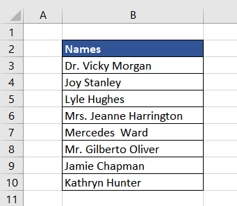
As a space separates the first and last name, we will use the same as a delimiter. The formula used will be as follows.

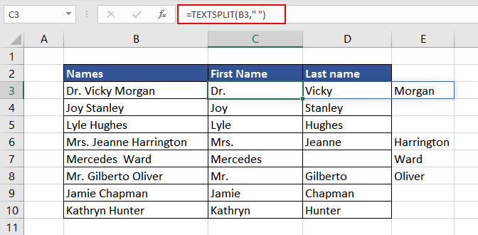
In the data above, a few names contain titles or honorifics, and they are also extracted as space is the common delimiter. Also, names such as in cell B7 contain extra space; therefore, an empty cell is returned. Let's make suitable changes in the formula to eliminate these flaws from our results.

To eliminate the titles such as Mr. and Mrs. from our final data, we can use them as delimiters. As we already know from the characteristics that to use multiple delimiters, we can pass them as an array in curly braces. The formula used will be as follows.

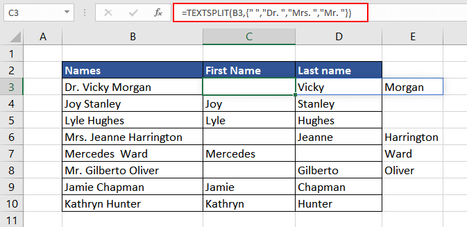
Although the titles were removed from the final data, the TEXTSPLIT function still returns an empty cell because it finds consecutive delimiters in the input text. To prevent that, we can set the value of the ignore_empty argument to TRUE. This way, the function will ignore the empty cells. The formula used will be as follows.

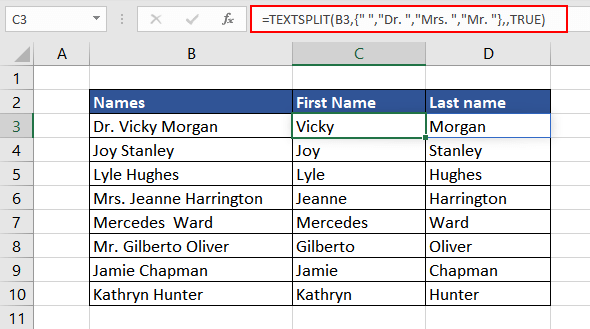
Now the data is clean and as required.

Example 4 – Separating a Date with TEXTSPLIT Function

Here, in this example, we have the holiday calendar for the year 2023. We now wish to segregate date, month, and year in separate columns to plan the vacations.

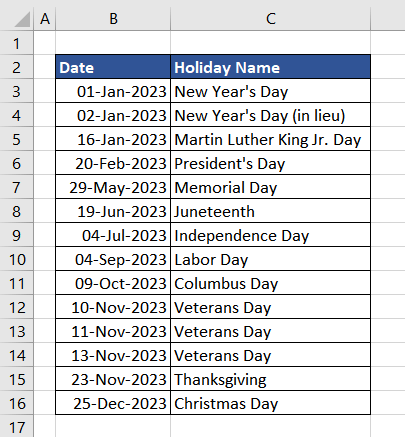
As the date separators are dashes (-), we will use the same as the col_delimiter. The formula used will be as follows.

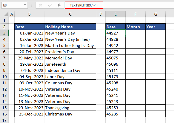
As observed in column E, the resulting data is different from what we expected. This is because the TEXTSPLIT function removes the date formatting of the input text and extracts the actual value, which is sequential numbers. We will use the TEXT function to ensure that the formatting remains intact.

We will convert the input date into the text format using the same date format, dd-mmm-yyyy, as in the data. The formula used will be as follows.

We will then use the return value of the TEXT function as the input value of the first argument (text) of the TEXTSPLIT function. The final formula to be used is as follows.

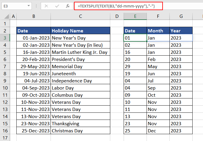
Now that we have the required information, it can be used further.

Example 5 – Understanding 'match_mode' argument of TEXTSPLIT Function

Here, in this example, we have received data on area dimensions which include length and width in feet. We now wish to segregate the length and width into separate columns for further data processing.

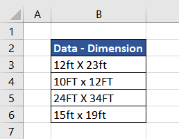
Using the TEXTSPLIT function, let's segregate the given data as per our requirements. As the letter 'x' is a separator, we will use that as the input value for col_delimiter.

The formula used will be as follows.

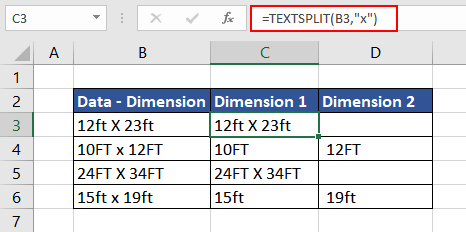
As the data is downloaded from the internet, there is a discrepancy with respect to the case type used. Some data contains 'FT' and 'X' in uppercase, while some have lowercase. The default nature of the TEXTSPLIT function is case-sensitive, which can be modified by altering the value of the match_mode argument.

To turn off case sensitivity, we can use 1 as the value for match_mode to ensure that the TEXTSPLIT function ignores the letter case. The formula used will be as follows.

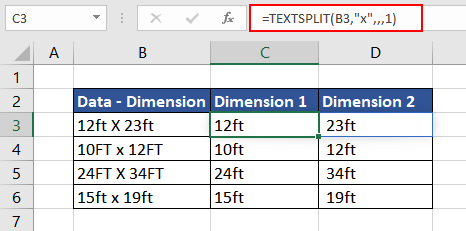
Now we have the required data. As mentioned in the characteristics, it can also be seen that when the value of the match_mode is set to 1, the resulting data is always in lowercase.

Example 6 – Extracting nth Word from a Text

Here, in this case, we have a list of quotes, and we intend to extract the third word from each quote. Using the TEXTSPLIT function, extracting the nth word from a text string will be incredibly easy.

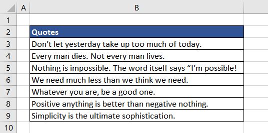
The TEXTSPLIT function will separate each word using space as col_delimiter, resulting in an array of values. The INDEX function then returns the value from the given location in that array. In this case, the location is 3. The TEXTSPLIT function to be used is as follows.

The resulting array will be the input value for the INDEX function, along with the location from which the word needs to be extracted. The formula used will be as follows.

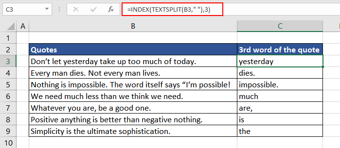
Now, we have the 3rd word from each given quote.

As the TEXTSPLIT function is a recent addition and is only available for Excel 365 users, practice on your own to discover different applications. We will bring you another interesting and useful function for you to fiddle with.