Excel LOOKUP Function – How To Use

The LOOKUP function allows us to easily retrieve required values from a given dataset. When working with large datasets, the function is extremely useful as it searches for a value within a given array or cell range and returns a corresponding value from the same position in another range.

The LOOKUP function offers two forms which are vector form and array form. The details of each are discussed further in the article. Beyond its functionality to look for an exact match, the function also offers to look for an approximate match.

Syntax

The LOOKUP function encompasses two different syntaxes and each one of them provides a distinct functionality. Depending on the nature of our data retrieval needs, we can opt for the syntax that provides greater flexibility in addressing different lookup scenarios.

The first one is called the vector form which accepts and deals with single array data. The syntax of the vector form of the LOOKUP function is as follows.

Arguments:

The vector form of the LOOKUP function is primarily used for simple one-dimensional lookups where we have separate columns/rows for lookup and result values. It accepts three arguments out of which two are mandatory.

'lookup_value' – This is a mandatory argument that accepts the value that we are looking for. The data in the lookup_value can be a variety of data types, including numbers, text, logical values, as well as names or references that point to specific values.

'lookup_vector' – This is also a mandatory argument as it contains the cell range or array where the LOOKUP function searches the lookup_value. Usually, the lookup_vector is a one-row or one-column cell range. However, if the input value includes more than one row or column, the LOOKUP function still considers the first row or column.

'result_vector' – This is an optional argument where the input value is a cell range which is ideally a single row or column range. As it is an optional argument, when it is left blank, the LOOKUP function returns the matched value found in When result_vector is defined, the function locates the match in lookup_vector and returns the corresponding value from the result_vector.

The second form of the LOOKUP function is called the array form. In this variant, the LOOKUP function finds the given value in the first column or row of the array and returns the corresponding value from the last column or row of the array.

The syntax of the array form of the LOOKUP function is as follows.

Arguments:

This form only accepts two arguments, and both are mandatory. The details of each are mentioned below.

'lookup_value' – This argument accepts the value that we wish to search for in the array.

'array ' – This includes the value of the array or cell range where we wish to search the lookup_value.

Note: One essential point to note about the lookup_vector and array arguments is that the LOOKUP function assumes that the data in the given arguments is arranged in ascending order. In the case of the array argument, if there is more than one row or column, the first column or row of the array must be sorted in ascending order.

Important Characteristics of the LOOKUP Function

One of the basic characteristics of the LOOKUP function is that it is case-insensitive. Other noteworthy features of the LOOKUP function are as follows.

• When the value in the lookup_value argument is smaller than the smallest value in the lookup_vector or first row or column of the array, the LOOKUP function throws a #N/A error.
• In another scenario, if the LOOKUP function cannot find the given lookup_value, it returns the closest smaller value within the array or lookup_vector.
• When using the array form of the LOOKUP function, if the array argument contains more rows than columns or an equal number of rows and columns, the function searches for the desired value in the first column. This essentially means that the LOOKUP function behaves like the HLOOKUP function.
• On the other hand, if the array argument includes more columns than rows, the function looks for the desired data in the first row which is a characteristic of the VLOOKUP function.

Although the LOOKUP function imitates features of the HLOOKUP and VLOOKUP functions, the latter two allow us to perform indexing both vertically and horizontally, while LOOKUP only returns the value from the last row or column.

Examples of LOOKUP Function

Let's start by using diverse inputs for the arguments of the LOOKUP function. This will help us grasp its fundamental functionality and both of its forms. Here we have taken a sample dataset that contains employee ID numbers, names, along with their ages (in years).

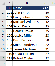
Let's take cell E1 which contains the data we are looking up. So, in this case, we are looking up Employee ID 105.

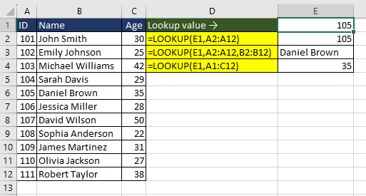
The first instance shows the vector form of the LOOKUP function when the optional argument result_vector is left empty. As we are looking for '105' in the cell range A2:A12, the function simply returns the matched value.

In the next case, the value of result_vector is mentioned. The LOOKUP function finds '105' in the given cell range and returns the corresponding value from cell range B2:B12 as "Daniel Brown".

The last instance showcases the array form of the LOOKUP function where it looks for '105' in the first column and returns the corresponding value from the last column.

Example 1 – Simple Use of LOOKUP Function

Imagine you are in the market for a new phone, and you have downloaded a price list of the latest models in an Excel spreadsheet. Your aim now is to explore the price details of the different models you are considering. This way, you can check if it fits your budget.

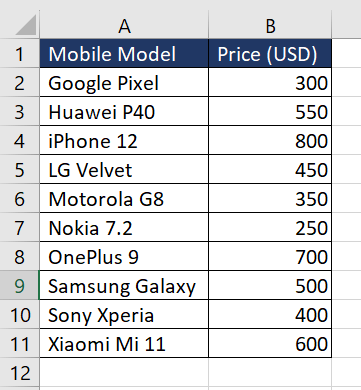
This is a classic case of the LOOKUP function which will allow you to search for a particular mobile phone model and retrieve its corresponding price. The formula used will be as follows.

The user can enter the lookup_value in cell E1. For instance, if we wish to check the price of "Samsung Galaxy", we will enter the same in cell E1. The LOOKUP function scans the cell range $A$2:$A$11 which is the Mobile Model column to find the exact match. Once the match is found, it will return the corresponding price (500 USD) for the model.

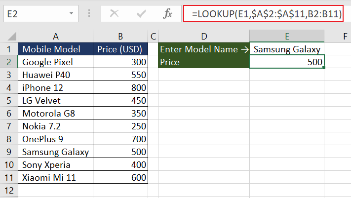
Now you can keep changing the model name in cell E2 and quickly retrieve the price. This will help you in your decision-making. Now, consider a scenario where you would like to perform a reverse lookup. Imagine you have a predetermined budget and are interested in finding out which mobile phone model has a price slightly below that budget.

We can use the LOOKUP function again. This time, it can be used to search for an approximate match in terms of price and return the mobile model that fits just under your specified budget. It is important to note that when the LOOKUP function does not find an exact match, it matches the closest smaller value.

We can ask the user to enter the budget in cell E4 and the formula used will be as follows.

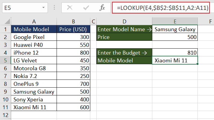
By entering 810 USD as the lookup_value in cell E4, the LOOKUP function searches for the mobile model that is equal to or less than 810 USD. In this case, it should return "iPhone 12" with a price of 800 USD, however, it does not.

The issue is the basic characteristics of the LOOKUP function that it assumes and necessitates that the value in lookup_vector is sorted in ascending order. Here, the lookup_vector refers to $B$2:$B$11 containing the prices. Let's sort the values and repeat the formula.

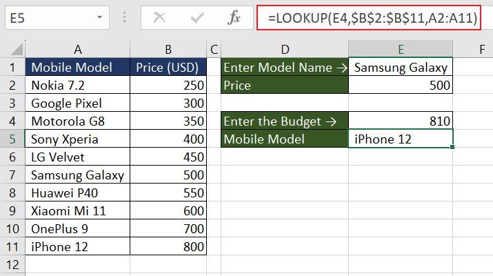
Now you have the correct return value.

As we are already aware, the LOOKUP function comes in two distinct forms. In the preceding example, we observed the functioning of the vector form. Let's delve into the array form of the LOOKUP function in the subsequent example.

Example 2 – Using Array Form of LOOKUP Function

Suppose we have the complete product details stored in an Excel sheet where each row in the dataset represents a different product, and the columns provide various attributes and characteristics of each product. Now, we wish to retrieve the product price based on the product ID.

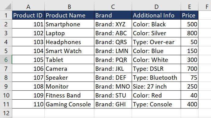
As we already know, in its array form, the LOOKUP function dynamically adjusts its behavior according to the dimensions of the array provided. In this case, the number of rows is more than the total columns, therefore the function looks for the lookup_value within the first column which is Product ID in our case. The return value will be data from the last column of the array, situated at the corresponding position matching the product ID which is the Price column.

This is a perfect case scenario to use the array form of the LOOKUP function. Let's take cell G1 where the user can enter the Product ID which will be the input value for the lookup_value argument. The formula used will be as follows.

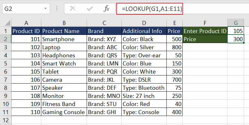
Although the LOOKUP function gave us the required value, it is recommended to use the VLOOKUP function or HLOOKUP function depending on the data especially since they do not require data sorting.

Example 3 – Identifying Latest Stock Prices with LOOKUP Function

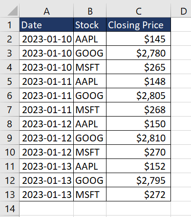
Suppose you are looking to invest in a few stocks and have been tracking the stock prices of three companies: Apple (AAPL), Google (GOOG), and Microsoft (MSFT). You have downloaded some historical stock data, including the date, and closing price for each trading day, which gets updated at the end of each day.

Now, combing through the data is tedious, therefore the goal is to easily find the latest closing price for any of these companies based on their stock name.

As we already know that one of the features of the LOOKUP function is when the lookup_value is not found in the lookup_vector, it returns the next value on the lesser side.

Additionally, the LOOKUP function operates under the assumption that the data is sorted in ascending order, therefore it returns the last value when the lookup_value is greater than all the values found in the lookup_vector. We will use this characteristic of the LOOKUP function to our advantage.

Let's take cell F1 where the user can enter the Stock name. Now, we will check if the value in F1 matches any value in cell range B2:B13.

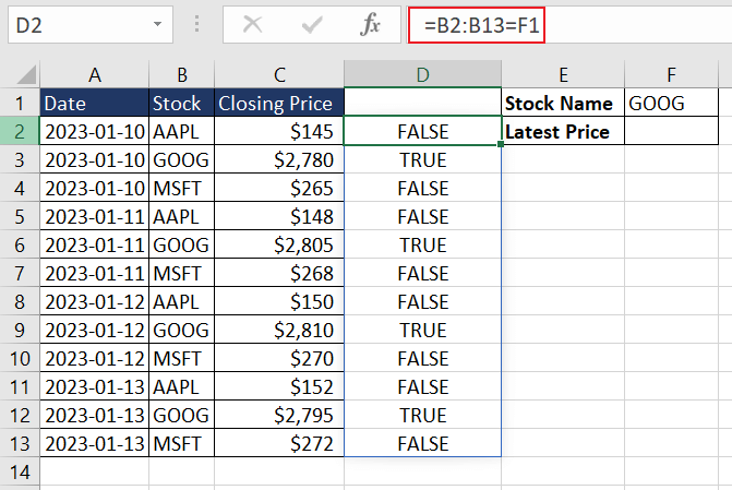
As we can see, we have an array comprising TRUE and FALSE values, signifying matches, and non-matches, respectively. By dividing 1 by the array, we get an array of 1s for matches and errors (#DIV/0!) for non-matches.

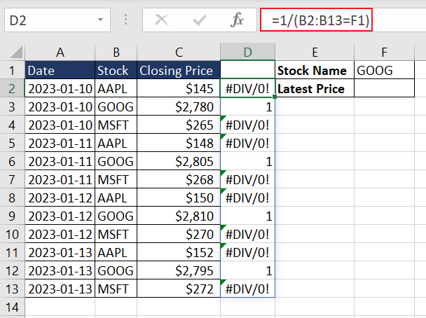
Now we use the above array as the input value for the lookup_vector argument. The next step is when the LOOKUP function searches for 2 in the above array.

Since it will not be found, it defaults to the last 1. This corresponds to the latest "GOOG" entry. The formula will be as follows.

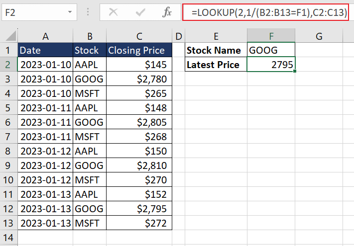
We finally have the latest closing price for "GOOG" which is $2795. The same logic can be applied to find the last non-empty cell in a column.

Example 4 – Finding Last Non-Blank Cell in Column

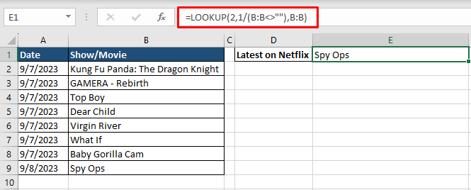
Lastly, one of the glories of the LOOKUP function is being able to find the last non-blank cell with it. Finding the last entry in a database can be useful for tracking stock prices (as we've seen in the prior example), weather conditions, delivery status, or (arguably the most important one) the latest show or movie on Netflix. Cue list:

Changing the condition in the lookup_vector, this is the formula we will use to find the last non-empty cell in Excel with the LOOKUP function:

The lookup_vector is set as 1/(B:B<>"") resulting in a spill array that gives us 1 for every row in the column that is a non-blank cell (first 9 cells are non-blank) and a #DIV/0! error for every blank cell.

With the lookup_value as 2, LOOKUP will default to its nature of returning the closest lesser value which as per LOOKUP's ascending order assumption will be the last 1 in the array, effectively the last entry in the dataset. With the last 1 chosen, the result_vector will be the corresponding value from column B (defined by B:B).

The final entry has been returned as "Spy Ops".

Now that you have a fair understanding of the LOOKUP function, it must be clear that it provides great functionality to streamline tasks such as data manipulation and data retrieval. Practice and identify more use cases of the function in your daily tasks. While you ace the LOOKUP function, we will work on another useful Excel function to add to your knowledge base.