How to Extract Only Numbers From a Cell in Excel

Quite the probable setup for disappointment if you came here thinking there's a straightforward, dedicated function in Excel to help rake the numbers out of alphanumeric data. Given that Excel is a fancy number dealer, we were fairly surprised too. All the more reason to explore, right? We're not pointing you anywhere but here!

A function may not be dedicated to the cause, but we are and we have 3 ways you can make numbers part way from your datasets. Do not be intimidated by the length of the formulas, (you only have to copy-paste, isn't that so?)

Any curiosity thirst will be quenched by the superfine minutiae of how the formulas work and alternatives to not having access to the later functions. We're going to crack this mystery and here's the cracker (or crackee, more like):

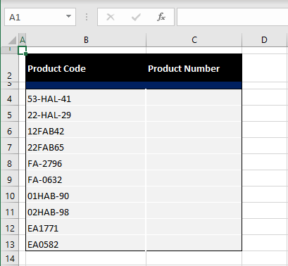
Column B holds product codes in alphanumeric style. And not a consistent one. You can see that the numbers are at both ends in some categories and at one end in others. Let's say Company A wants to homogenize the codes for smooth data entry and readability of sales records.

Yes, number extraction is the mine work for today and the usual methods like Text to Columns cannot work because we're not dealing with a single format here.

All three methods given in this tutorial, as you will observe, can work on extracting numbers from values whether the numbers are interspersed or in different formats.

Extraction goggles on, let's go!

Method #1 – Using TEXTJOIN Function

Use the TEXTJOIN function to only extract numbers from a cell's value in Excel. The TEXTJOIN function combines a range of text strings. While that sounds like the converse of wanting to separate numbers, in effect, the TEXTJOIN will be used to concatenate the numbers dispersed in a text string.

Word of caution, skip to the next section if your Excel is older than 2019 or you are sans MS 365 subscription since the TEXTJOIN function is only available for the mentioned.

So now we make alphabetic strings disappear? Somewhat, yes. Find out how the formula below returns just the numeric part of a text string with the TEXTJOIN function:

Firstly, the ROW and INDIRECT functions are used to generate a spill series of numbers from 1 to the number of characters in B4 (measured by the LEN function). LEN counts the number of characters as 9 in this case. The & operator makes this expression 1:9. The ROW function is used to return a row number and will take the reference from the INDIRECT function, making the spill values 1 to 9.

Then the MID function returns 1 character of B4 for every number spilled by the ROW and INDIRECT functions e.g. 1 returns the first character of B4 as "5", 2 returns the second character as "3". Therefore, this part of the formula returns the entire text string in B4 as a spill, readying each character to be checked separately as a number.

The IFERROR function loops through every character and multiples it by 1. The theory is that the numeric content of the spilled values can be multiplied by 1 and will return as they are.  A letter of the alphabet cannot be multiplied and will return an error.

When faced with an error, the IFERROR function will return blank text "", ruling out the entire alphabetic string. What is left are the numbers and blank cells. Finally, the TEXTJOIN function collates the numbers by joining (without a delimiter) all the values left in the spill range, ignoring blank cells (set by "TRUE" in the second argument).

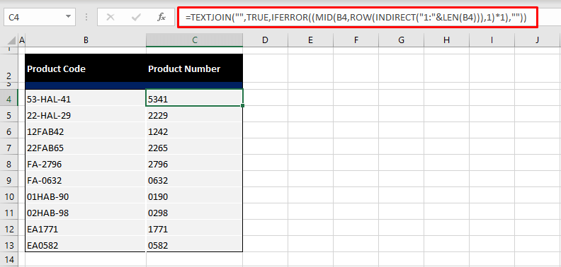
Note: After typing the whole formula, (for Excel 2010 – 2019), enter this array formula with the Ctrl + Shift + Enter keys. MS 365 users can just hit the Enter key as with regular formulas.

Method #2 – Using Custom Formula

Extract just the number component from a cell in Excel with the help of a formula. As mentioned, this formula is an alternative for non-Excel 2019 or MS 365 users since earlier Excel versions do not support the TEXTJOIN function.

The base of this formula is the same as the one above up until the MID function but additionally requires the IF, SUM, SUBSTITUTE, SUMPRODUCT, LARGE, INDEX, ISNUMBER to get similar results.

Since this takes up a little more space (subjectively) than other formulas, we'll break it down bit by bit. This is the formula, and the explanation follows:

Breakdown:

For explanatory purposes and to tie everything in later, we'll call this section of the formula "core calculation". It starts with the number series by the ROW and INDIRECT functions and ends with the SUMPRODUCT function so here we go.

Again starting with the ROW and INDIRECT functions, a series of numbers is generated from 1 to the number of characters in B4 which is 9. The ROW function places the consecutive numbers for the reference returned by the INDIRECT function. We get 9 rows of spilled number series starting from 1 like so: {1;2;3;4;5;6;7;8;9}

Every number in this series is the starting point for the MID function for returning 1 character from the value in B4 as: {"5″;"3″;"-";"H";"A";"L";"-";"4″;"1"}

Then there's the ISNUMBER function to check each character from the MID function as a number and return TRUE or FALSE:
{TRUE;TRUE;FALSE;FALSE;FALSE;FALSE;FALSE;TRUE;TRUE}

Adding the double unary operator converts these Boolean values into 1 and 0 respectively, prepping to operate as an array formula for the INDEX function. Multiplying these 1s and 0s with the number series generated by the ROW and INDIRECT functions will give us the position of the numbers in the cells, the other characters will result in 0.

{1;2;0;0;0;0;0;8;9}

The LARGE function returns the kth largest value. K here is the number series from 1 to 9. Hence, we get INDEX's output in descending order. This will stack the zeros to one side, getting the position of the numbers together.

{9;8;2;1;0;0;0;0;0}

The value the MID function is using to return characters is 0&B4, joining 0 to B4's value as the MID function returns the characters as per the defined positions (shown above). This added 0 and +1 as MID's second argument will help avoid the #VALUE! error which will arise when MID is to return the 0th position from B4. As of now, the 0th position will become 0+1 i.e. the 1st position which will return the concatenated 0.

{"1″;"4″;"3″;"5″;"0″;"0″;"0″;"0″;"0"}

Here's the masterstroke that begins flipping things around. This part of the function places a regular 10 and raises it to a power. The exponent is fed by the number series by ROW and INDIRECT going like 10¹, 10², and so on resulting in:
{10;100;1000;10000;100000;1000000;10000000;100000000;1000000000}

Divided by 10 and we’re at:
{1;10;100;1000;10000;100000;1000000;10000000;100000000}

You can see at the end of the formula that the "10" expression has been multiplied by the MID function and will result in: {1;40;300;5000;0;0;0;0;0}

This is where the core calculation ends. Have it known that we've tried the SUM function in place of SUMPRODUCT with no problems. Anyhow, when the SUMPRODUCT function adds it up, we get (hallelujah) 5341 which is what we're looking for and you can very well stop here as the formula works fine to separate the numbers from a string and return them:

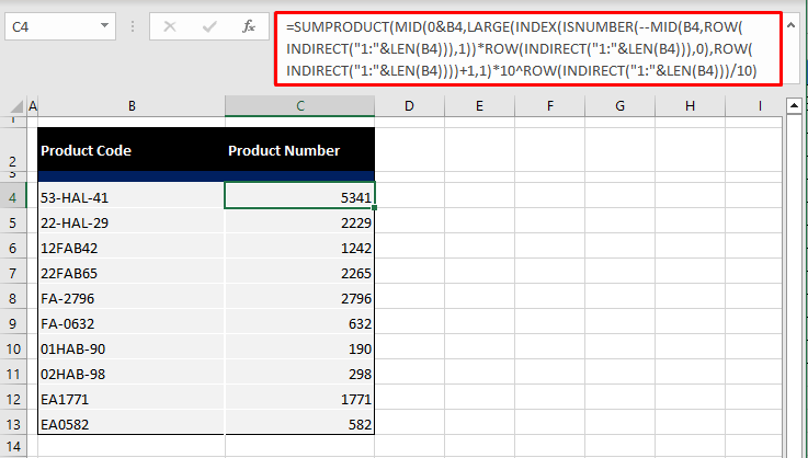
The hitch arises if your input range also contains values that don't have any numbers. Let's show you what happens:

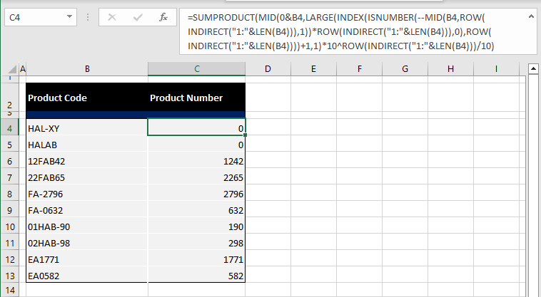
We've changed the top two product codes to be without numbers and the formula returns 0. The only problem is that the 0 can be mistaken to be the only number in the code. In that case, let's use the complete formula to give us empty text when there are no numbers in the input string. Moving on to further breakdowns.

Now the SUBSTITUTE function will replace any occurrence of the digits 0 to 9, one by one, in B4 with a blank space. This will spill in a horizontal range. Since B4 doesn't have any 0s, B4 will be returned as is. B4 does have the number 1 and so in the second value of the output, 1 will be replaced by a blank space. In this way, all the digits will be checked:
{"53-HAL-41″,"53-HAL-4″,"53-HAL-41″,"5-HAL-41″,"53-HAL-1″,"3-HAL-41″,"53-HAL-41″,"53-HAL-41″,"53-HAL-41″,"53-HAL-41"}

The LEN function counts the number of characters in each value of the spilled result. With no 0, we had all 9 characters in the first value. In the second value, 1 was replaced by empty text, leaving 8 characters and so on.

{9,8,9,8,8,8,9,9,9,9}

Subtract this result from the total number of characters, again counted by LEN. We get the number of missing characters and thus the count of numbers present in B4.

{0,1,0,1,1,1,0,0,0,0}

To bring the tally together, the SUM function will suffice and result in 4.

And at last, the complete formula is brought together by the IF function. In plain words, the formula says that if the count of numbers is not greater than zero, return empty text (see the last argument of the formula). If the count of numbers is greater than zero, perform core calculation. Since the count of numbers in B4 is 4 and is greater than 0, the core calculation has landed us at the final output which is 5341.

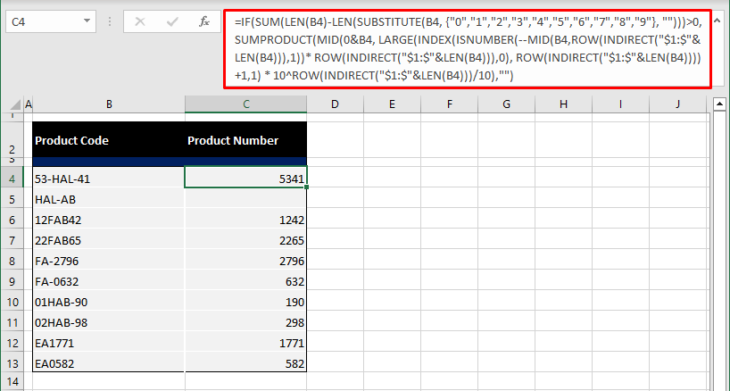
B5 as shown above does not have numeric data and results in a blank cell now.

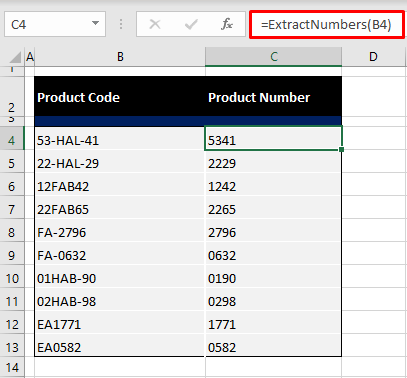
Pro tip: Notice we have a few instances with only 3 digits extracted as Excel automatically eliminates leading zeros from numbers. A quick solution is to add the TEXT function to the formula so we can have the leading zeros without default removal. Use this formula to extract numbers from a cell and keep leading zeros:

The TEXT function has been added and the format we have supplied is "0000" to keep the resulting number at 4 digits even if it leads with 0s.

Method #3 – Using VBA

Learn how to extract only numbers from a cell using VBA in Excel. VBA programming is used to automate tasks in Excel. By now you would know that there is no direct function in Excel that can get this job easily done for us. Thus, we shall plant a function on our own!

Using a code involving the IsNumeric function in VBA, we will set up a function to extract numbers from a range of text strings. The following steps will demonstrate in complete detail how to utilize VBA to get only numbers from a cell:

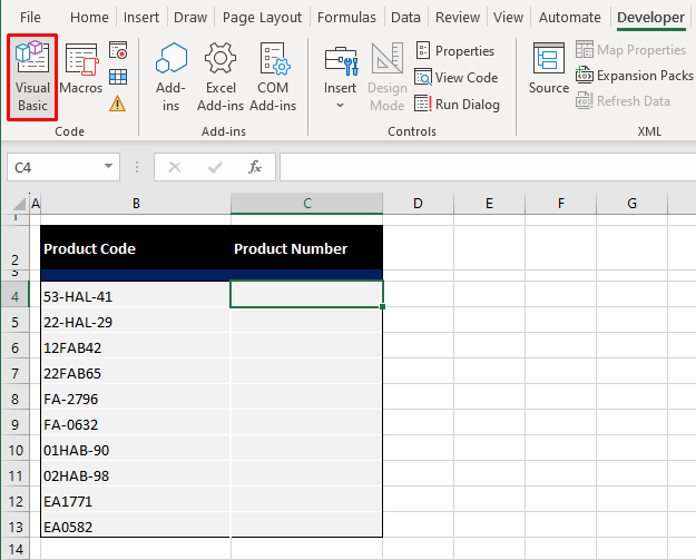
• Open the Visual Basic editor by pressing the Alt + F11 If you have the Developer tab enabled, you can also use the Visual Basic button in the Developer tab's Code group.
• 
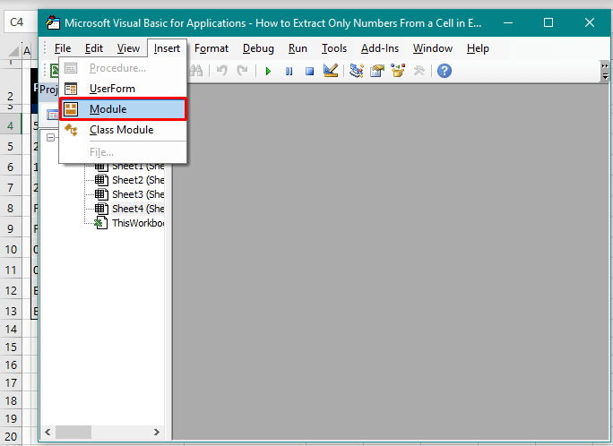
• In the editor, click on the Insert tab and select Module from the drop-down menu.
• 
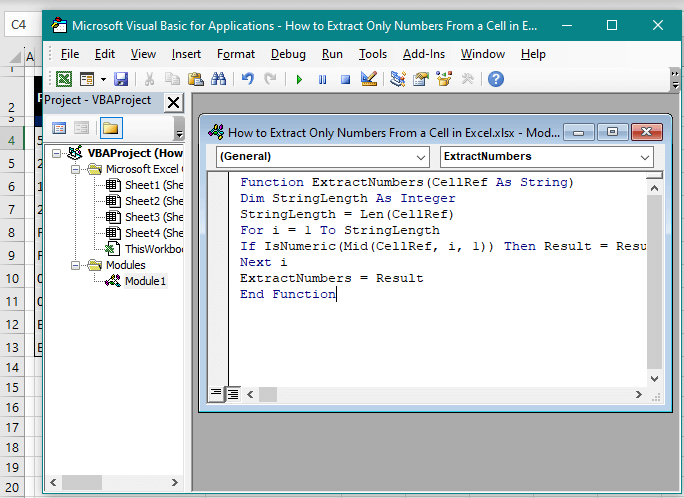
• Copy and paste this code from below in the Module window:

• Function ExtractNumbers(CellRef As String)
  Dim StringLength As Integer
  StringLength = Len(CellRef)
  For i = 1 To StringLength
   If IsNumeric(Mid(CellRef, i, 1)) Then Result = Result & Mid(CellRef, i, 1)
   Next i
  ExtractNumbers = Result
  End Function

  The code uses the Mid function to operate with the IsNumeric function in VBA to extract numbers from within a cell's value. The function name in the first line of the code ("ExtractNumbers" in this case) is the name you will use on the worksheet so be mindful of that.

• After inserting the code, close the Visual Basic
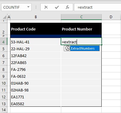
• Enter the function name in the target cell on the worksheet and it will show up in IntelliSense.
• 
• Select the function and refer the cell containing the text string you want to extract numbers from.

Enter the function and it will extract the numbers from the relevant cell:

And that readers, is how numbers are extracted from a cell in some handy Excel ways. More handyman Excel services are coming up your way giving you all the fine tools to chisel your way through with just the perfect Excel trick. Ready? Tricky? Go!