How to Find Max Value in Range in Excel (5 Easy Ways)

Alright, down the magnifying glasses, we're here to make speedy decisions that require speedy solutions. Finding the topmost value is a concept that would not be alien to you and it is all too easy for Excel too. An extreme value is an indicator, shows the distribution of values in a dataset, highlights top performers, and enables conditional analysis.

If you were tasked with identifying the largest number from the small lot shown below, you'd probably come to the correct conclusion within seconds:

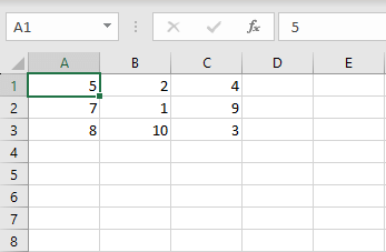
If we were to double or triple this lot, you still might be able to detect the highest figure but not within the same number of seconds. And with increasing numbers, the task will quickly become subject to human error. Take the following case example where there are hundreds of rows of data:

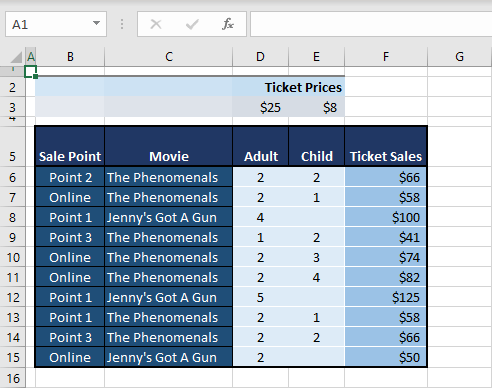
We have sample sales data here of a cinema chain and the simple objective is to find the maximum value in ticket sales. Tools like the MAX function are specifically designed to make seamless work of finding a range's highest value in Excel. Or you can proceed with the MAXIFS, LARGE, SUBTOTAL, and AGGREGATE functions for some strings attached. What strings? You'll find out in this tutorial.

Note: The methods below for finding the maximum value will work for numbers as well as dates and time.

Let's max out on Excel madness!

Method #1 – Using MAX Function

Find the maximum value in a range using the MAX function in Excel. The MAX function returns the largest value from a set of values. We will apply the MAX function to the number part of the dataset in our case example to obtain the largest value of ticket sales by a customer. The formula we'll be using with the MAX function is as follows:

The MAX function is used here with a single argument, that is the range from which we want the maximum value picked out. The range is F6 to F15 as per our case example. The formula returns $125 which is the highest value of ticket sales in the dataset for a single instance.

Note: If you have continuous rows of data (e.g. F6:H15) and only want the values in columns F and H checked, you can get the MAX function to take just the two columns, separated by a comma in the formula like so:

And as simple as that, you have the maximum value all figured out. Then what do you do if there are a couple of spanners to be thrown into the works? Say you want the highest value only from online sales. We point you to the solution below!

Method #2 – Using MAXIFS Function

Use the MAXIFS function in Excel to find the maximum value in a given range. The MAXIFS function applies the set conditions to a range and returns the maximum value therein, falling under those conditions.

That is the perfect opportunity for us to narrow the search to only online sales. MAXIFS is an alternative to applying filters to the dataset where you feed the filter requirements into the conditions in the function.

Have a go at the formula below that hosts the MAXIFS function to find the highest value in a range:

The formula starts with the range of values that we want to check for the maximum value which is F6 to F15 in this case. E18 in the third argument indicates the condition; we want to find the online proceeds and therefore the value "Online" from the first column of the dataset.

We have hence entered the range B6:B15 in the second argument. Instead of using the cell reference E18, you can enclose the text to be searched in the formula in double quotes like this "online". The formula would then be:

Overall, the formula will check for "Online" in column B. From all the values in column F, the largest number that corresponds to being an online sale will be returned and that is $82.

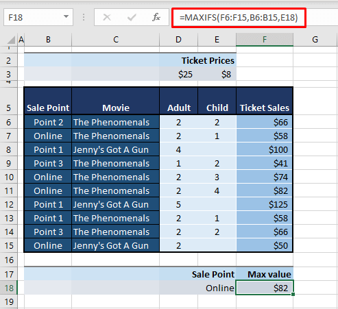
Likewise, multiple conditions can be defined for their criteria and the relevant range. For example, you want to view the highest online proceeds for a particular movie. The formula below shows the added condition:

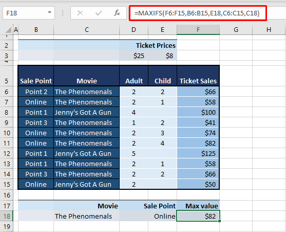
We now see two more arguments in this formula. One is C6:C15 which is the range for searching the second condition. The second condition is C18 (the movie "The Phenomenals") which is the search value. Now MAXIFS will return the maximum value of The Phenomenals' online sales.

Method #3 – Using LARGE Function

Identify the largest value in a range using Excel's LARGE function. The LARGE function returns the k-th largest value in a range. As required, we can use the LARGE function to spot the largest or 2nd largest number in a dataset. Use the given formula as a base to apply the LARGE function for finding the greatest value in Excel:

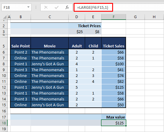
The function has taken the range with the numbers. The only thing left is to provide the k figure for the function to return the kth value. The largest number would mean the 1st number in this example case and so the value of k is 1 here (as shown in the second argument). See how it works applied to the sample dataset:

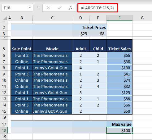
Now to get the 2nd largest sales figure instead, the second argument will be entered as the number 2.

The formula returns the second greatest value as $100 in the range F6:F15.

Method #4 – Using SUBTOTAL Function

Discover the highest value within a specified range in Excel utilizing the SUBTOTAL function. The job of the SUBTOTAL function is to return a total of a subcategory in a dataset. While we don't require a subtotal per se, it is another feature of the function put to purpose here and it is usage with filters or hidden rows.

This time, we have filtered the dataset to show only the online ticket sales (see below). Now if we apply the MAX function to attain the highest value, we get $125.

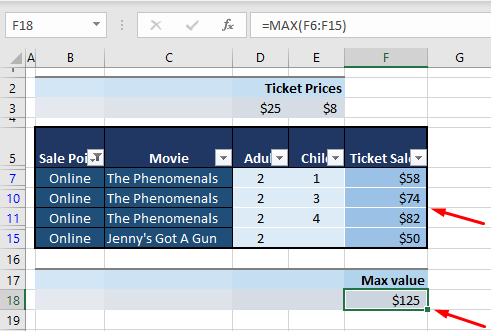
Have you noted that isn't right? We should not be getting $125 as we can't even see this value in the filtered data. Filtered data requires a different set of functions and one of them is the SUBTOTAL function.

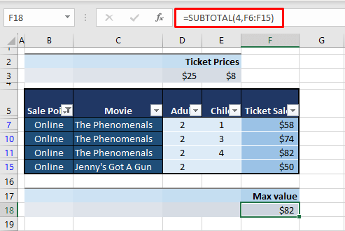
This will pick out the target value only from the filtered bunch, using the MAX function from its function options. Read the details and the formula below:

The first argument in the formula is 4 which is the function number designated to the MAX function in SUBTOTAL's function options. Excel's Formula AutoComplete will help you out here as you type:

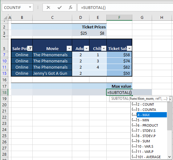
The second argument is the range containing the numbers which is F6 to F15. That is how the SUBTOTAL function uses the MAX function to find the maximum value in filtered data.

Method #5 – Using AGGREGATE Function

The maximum value in a range can be found with Excel's AGGREGATE function. The AGGREGATE function returns an aggregate in a dataset. Take it as the big brother of the SUBTOTAL function; SUBTOTAL with more options. Carrying forward our case example, we can use the AGGREGATE function to apply the LARGE function on filtered data. The formula below will explain everything:

14 in the first argument is the function number of the LARGE function. 7 in the next argument is the option to "ignore hidden rows and error values". Without ignoring hidden rows, we would be back to the problem of including the values that are filtered out.

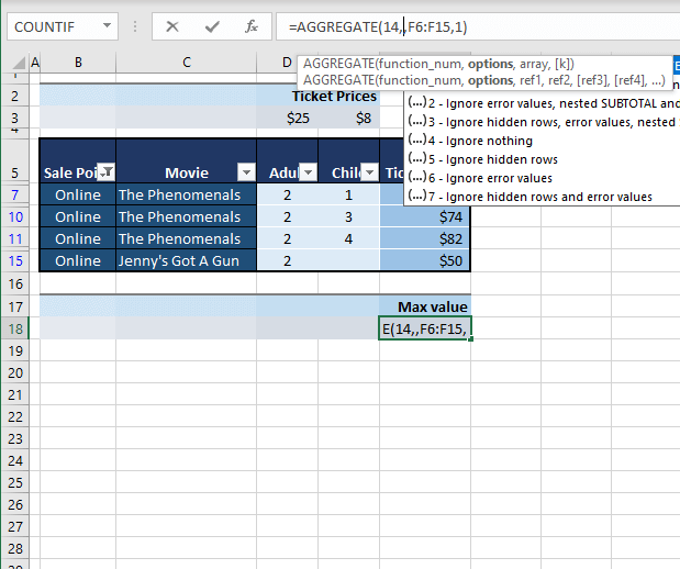
Next is the range AGGREGATE needs to work on (F6:F15). The last argument is 1 which is the kth value that comes along with using the LARGE function and for the largest number, k is 1.

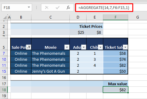
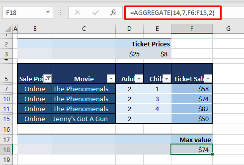
And again, if you're going with the LARGE function in AGGREGATE, you are probably doing it for one of the extra options or for finding the kth value. Thus, here is a sample formula for finding the 2nd largest value in line with our case example:

1 has been replaced with 2 in the last argument and the results are as follows:

Now you can find a range's maximum value in Excel at the drop of a hat, and it will quickly help you analyze the data with regard to the top value. We'll be back to pull more rabbits out of the grand hat called Excel. Ready? Tricky? Go!